Adaptation of a Large Language Model for a Specific Task using Parameter Efficient Fine-Tuning

GaMS LoRA tuning and batch inference

Opis

This pipeline provides code and a set of instructions on how to adapt a large language model to a specific task, e.g., detecting sentiment of user input, categorizing internal documents, or building a question answering system based on a specific set of documents. It is suitable for many domains such as healthcare, legal services, and museums, and enables language understanding and generation. The prerequisites are a modest amount of task-based data, either annotated texts or a set of input-output pairs. The pipeline first helps users in preparing data for fine-tuning, and then provides the know-how and code for fine-tuning the model with the prepared data. Finally, it provides code for efficient inference using the fine-tuned model. A worked example of fine-tuning is provided. The pipeline uses the Slovene large language model (LLM) GaMS as well as other state-of-the-art open multilingual LLMs and libraries that support LLM fine-tuning with LoRA and QLoRA, and efficient inference with vLLM.

Pričakovani rezultati

Following the resources provided in this service, reader will be able to: (1) Set up a working environment on a HPC cluster; (2) Convert the training data into the format expected for SFT training; (3) Perform SFT training using Transformers and TRL libraries; (4) Use LoRA adapters during the training and freeze the base model using the PEFT library; (5) Deploy the training across multiple GPUs and nodes on a Slurm based cluster; (6) Optimize the training through using Flash Attention, DeepSpeed, Gradient checkpointing and Liger kernel; (7) Monitor the training process using the WandB platform; (8) Merge LoRA adapters back into the base model after the training; (9) Perform a large scale offline batch inference using vLLM.

Kartica storitve

Kategorija	AI development and deployment
Domena	Natural Language Processing, Domain Adaptation
Vertikala	Cross-domain
Ciljni uporabniki	SMEs, Enterprises, Public Sector, Scientific Users
Tip storitve	Pipeline
Rezultat	Task-adapted model for training; generated text for inference
Zahteve	Requires NVIDIA GPU node
Preizkušene platforme	HPC Vega
Omejitve
Na voljo od	Q2/2026
Licenca	MIT
Slika
Oznaka slike
Repozitorij	GaMS-PEFT-Tuning

Introduction

Large language models are becoming essential for task automation. Open-source models are especially important, as they can be run on premise, ensuring your data remains private. This is important when you want to protect your intellectual property or work in domains where data protection is essential (e.g. healthcare, public sector, law, etc.). Even though such models are trained to perform well on a wide variety of tasks, they might fail to reach near-optimal performance on a specific task, which is often required to implement such pipeline in production. This is where fine-tuning kicks in - we can improve the model's performance on the desired task by training it using a parameter efficient approach such as LoRA. This service provides the code and knowledge for task specific fine-tuning and large-scale inference, which is essential when we need to process a large amount of documents.

The service consists of two parts:

1. A GitHub repository containing the code for running the LoRA SFT Training and vLLM inference on Slovene HPC Vega.
2. This book containing detailed explanation of the code and approaches used in this service.

GaMS

GaMS (Generative Model for Slovene) is a family of large language models developed within the PoVeJMo project. The models are open-source and specialized for Slovene language. Their weights are openly available on the HuggingFace portal under the CJVT organization. The models are based on Google's Gemma and exist in several versions - they vary in the number of parameters, starting model (either Gemma 2 or Gemma 3 and Gemma 4 in the future) and the training stage (Instruct versions are instruction-tuned and ready for immediate prompt-completion usage and the versions without Instruct in their name are only pretrained and have to be fine-tuned for specific tasks). Since the models are middle-sized ("useful" versions range from 9 to 27 billion parameters), they are suitable for task-specialization through fine-tuning (they do not require a lot of compute resources). Therefore, they are perfect for this service.

Book content

This book walks through the fine-tuning and inference pipeline. Each chapter builds on the last, but the pipeline's modular design also means that a reader already familiar with, say, data preparation can enter at the training chapter without loss of context. Whatever your starting point, the goal is the same: a clear, principled understanding of how large language models are adapted — not just that it can be done, but why each piece of the process is designed the way it is.

We begin with the practicalities of setting up the computational environment — managing dependencies, configuring distributed training, and ensuring that every step of the workflow can be reproduced faithfully on a high-performance computing cluster. From there, we move into data preparation: the principles behind the tokenization and the SFT data format.

The training chapter is the technical heart of the book. We examine how LoRA is configured and applied, how the Hugging Face TRL, PEFT and Transformers libraries orchestrate the training loop, how DeepSpeed splits the model across GPUs and how we monitor the training process. Following the training, we explain LoRA merging process and provide the code for merging.

In the final chapters we first address the batch inference using vLLM library. We show how to distribute the inference across multiple nodes to speed up the process. Finally, we provide the script for quick data inspection to see what we achieved with our pipeline.

Environment Setup

Before we start with the training, we need to set up our environment. This includes cloning the code from GitHub and installing the necessary libraries.

Cloning the Repository

The code is available at the GaMS-Team/GaMS-PEFT-Tuning repository. We assume you have SSH access configured for your GitHub account (if you don't, use the HTTPS link under the clone button at the repository) and that git is available in your environment (it will be on virtually any cluster):

git clone git@github.com:GaMS-Team/GaMS-PEFT-Tuning.git
cd GaMS-PEFT-Tuning

All subsequent paths in this service description are relative to this repository root.

Installing the libraries

We will pack our environment into an Apptainer image. Apptainer (former Singularity) is a container system used by the Vega supercomputer. Most of the EuroHPC clusters use similar container system.

Building the Container Image

We will build the Apptainer image from the recipe. The recipe file lives at apptainer/recipe.def, and we will write the resulting image to apptainer/slaif_peft.sif.

The standard build command is:

apptainer build apptainer/slaif_peft.sif apptainer/recipe.def

This command instructs Apptainer to process the recipe definition, pull the base CUDA image (defined at the beginning of the recipe), run all the installation steps defined in the %post section of the recipe, and write the final image to the specified .sif path.

Once the build completes, apptainer/slaif_peft.sif contains the entire reproducible environment as a single file. This file is what all of our Sbatch scripts will reference when launching training and inference jobs. The environment it encapsulates will behave identically whether the job runs on one node or sixteen, and whether it runs today or two years from now on a different cluster — as long as the .sif file is present.

Fakeroot issue

On many HPC clusters, building containers requires fakeroot mode, which allows unprivileged users to simulate root ownership during the build process without actually having root access. Whether fakeroot is required depends on how your cluster's Apptainer installation is configured — some clusters enable unprivileged builds by default through kernel user namespace support, while others require fakeroot explicitly. If the standard build command fails with permission errors, the fix is simply to add the --fakeroot flag:

apptainer build --fakeroot apptainer/slaif_peft.sif apptainer/recipe.def

In order to build with the fakeroot mode, you have to be added into the fakeroot usergroup. You may need to contact the system administrator to add you to the group. Other altenratives are building the image on another Singularity/Apptainer cluster, where you have the permissions or building a Docker image on your local computer. You can then provide the Docker image to the Apptainer and it will convert it to the .sif file.

The Software Stack

The container we build is defined by apptainer/recipe.def and starts from NVIDIA's official CUDA development image, specifically nvidia/cuda:12.8.1-cudnn-devel-ubuntu24.04. Building on top of this official base image means we inherit a properly configured CUDA 12.8.1 installation with cuDNN, the deep neural network primitive library, already present. We then layer our Python environment on top of this foundation.

1. PyTorch 2.9.1 is the centerpiece of the stack. We pin this version explicitly because FlashAttention 2, DeepSpeed, and vLLM all have specific compatibility requirements with PyTorch's internal C++ ABI, and the combination we have validated is PyTorch 2.9.1 with CUDA 12.8.

2. Hugging Face Transformers 4.56.1 provides the model architecture implementations, tokenizers, and the configuration classes that describe GaMS and similar causal language models. TRL 0.25.1 (Transformer Reinforcement Learning) sits on top of Transformers and provides the SFTTrainer class that orchestrates our supervised fine-tuning loop — handling packing, dataset formatting, and integration with PEFT adapters. PEFT (Parameter-Efficient Fine-Tuning) is the library that implements LoRA itself, providing the LoraConfig and the adapter injection logic that modifies the base model without touching its original weights.

3. DeepSpeed 0.18.1 is our distributed training engine. It implements ZeRO (Zero Redundancy Optimizer), the memory optimization strategy that allows us to train models whose parameters, gradients, and optimizer states would not fit on a single GPU by sharding these tensors across all GPUs in the job. We discuss DeepSpeed in detail in the training chapter, but from an environment perspective it matters because it includes compiled CUDA extensions that must match our CUDA version exactly.

4. FlashAttention 2 replaces PyTorch's standard attention implementation with a memory-efficient, IO-aware algorithm that substantially reduces both memory usage and compute time for long sequences. Since we train with sequences up to 16,384 tokens, standard attention would be prohibitively expensive; FlashAttention 2 makes it tractable. Liger Kernel complements this by providing fused kernel implementations for other common operations in the Transformer forward pass — RMSNorm, RoPE embeddings, SwiGLU activations — reducing memory fragmentation and kernel launch overhead. As the FlashAttention installation can take up to few hours due to the kernel compilations, we install it from the prebuilt wheel (we need to be careful to use the wheel that matches our Python, PyTorch and CUDA versions).

5. vLLM 0.16.0 serves a different phase of the pipeline entirely. Where the training components are needed during fine-tuning, vLLM is our inference engine used during batch evaluation after training is complete. It implements PagedAttention, a KV-cache management strategy that dramatically improves throughput for batched generation, and it supports tensor parallelism across multiple GPUs for accelerating inference on large models.

6. Finally, WandB (Weights and Biases) provides experiment tracking. Every training run reports its metrics — loss curves, learning rate schedule, gradient norms — to a WandB project, giving us a persistent, searchable record of all experiments regardless of which cluster node they ran on.

Data Preparation

The data preparation stage is the most important part of the fine-tuning process. For the supervised fine-tuning we need to prepare the data in the prompt/response format - each example consists from the input to the model and the expected output. Through the training examples we teach the model both how to solve the task and how to format the output.

This is why the preparation of the fine-tuning dataset matters. It is not merely a collection of examples the model memorizes; it is the curriculum through which the model internalizes new behaviors. If the dataset is noisy, the model learns noise. If it lacks diversity, the model overfits to surface patterns. If the format is inconsistent, the model learns inconsistency. Building a clean, well-structured dataset is therefore not a preprocessing chore to be rushed through before the training.

Since the point of this service is not to produce a pipeline for task or domain specific data extraction or creation, we take an existing fine-tuning dataset. We use the GaMS-Instruct-MED 2.0, dataset, that is publicly available. We show how to prepare the dataset for supervised fine-tuning.

Demo Dataset

The GaMS-Instruct-MED 2.0 Dataset

GaMS-Instruct-MED 2.0 is a Slovenian-language medical instruction dataset designed specifically for supervised fine-tuning of instruction-following models. It consists of two components that are stored in separate files and are joined during preprocessing.

The primary file, GaMS-Instruct-MED_2.0.json, contains the instruction/response pairs. Each record carries a unique identifier (id), an instruction field containing the task description and instructions, input containing the specific question, an output field containing the expected assistant response, a type field that categorizes the example, and an optional context_id field that, when present, links the example to an external passage of text from the second file.

The second file, GaMS-Instruct-MED_2.0_context.json, is a collection of context passages. Each passage is identified by a context_id that matches the corresponding field in the primary file. These passages are chunks of reference texts that provide the grounding a model needs to answer certain questions accurately.

The presence of the context separates two different task types. For the questions without the context, the model needs to rely on its own internal knowledge that is stored in the model parameters. But other questions are grounded in specific source documents and the correct answer depends on the content of that document. This is precisely the behavior we want in a retrieval-augmented generation (RAG) setting, where a retrieval system fetches relevant documents at inference time and the model must use them intelligently.

Downloading and unpacking the data

The dataset we use is publicly available on CLARIN.SI repository, where it was published by the group of researchers from Better, who developed the dataset during the Povejmo project. We need to first download and unpack the data. We can do it using the following series of commands (run them inside the root directory you cloned from GitHub):

mkdir data/
cd data/
curl --remote-name-all https://www.clarin.si/repository/xmlui/bitstream/handle/11356/2045{/GaMS-Instruct-MED_2.0.zip}
unzip GaMS-Instruct-MED_2.0.zip
cd ..

The script first creates a new dir called data, downloads the files from the CLARIN.SI directly into the newly created folder and unpacks the content of the downloaded zip file. After extraction, your data directory should contain:

data/
└── GaMS-Instruct-MED_2.0/
    ├── GaMS-Instruct-MED_2.0.json
    └── GaMS-Instruct-MED_2.0_context.json

Preparing Model Training Data

Behind the SFT Data Format

Before describing the transformation pipeline itself, it is worth pausing on a conceptual point that is easy to overlook but fundamental to how supervised fine-tuning works: the distinction between the prompt and the completion, and why that distinction exists.

During the pretraining, the model is trained to predict each token given all preceding tokens. During the SFT phase, the model's tokenizer first converts the conversation into a single sequence using a chat template. The model is then again trained to predict the next token given the previous ones. However, training on a full conversation would mean that the model receives a loss signal on every token — including the tokens that make up the user's question. The model would learn not just to produce good answers, but to predict what questions look like. This is problematic as generating a question and following an instruction are not the same cognitive operation, and training the model to do both from the same loss signal blurs the boundary between them. In practice, models trained this way tend to be worse at sticking to the answer role; they may repeat the question, generate another one or fail to produce the expected answer.

The solution is straightforward: we split each training example into a prompt (everything up to and including the user's question) and a completion (the assistant's response), and we compute the training loss only on the completion tokens. The prompt tokens are fed forward through the model to build up the correct hidden state, but their predictions do not contribute to the gradient update. The model is penalized only for failing to produce the correct answer, not for failing to predict the question. This is the defining feature of supervised fine-tuning as opposed to continued pretraining, and it is what makes SFT so effective at teaching instruction-following behavior.

In practice, this is implemented by creating a loss mask with 1 for completion tokens (telling the loss function to compute the loss on these tokens) and 0 for the preceding tokens (telling the loss function to ignore these tokens). The TRL library's SFTTrainer, which we use in this service, handles this automatically when examples are provided in the standard prompt-completion format, as we will describe shortly.

The Transformation Pipeline

The script prepare_data/transform_and_split.py takes the two raw JSON files and produces three JSONL files ready for training. It accepts the following arguments:

python prepare_data/transform_and_split.py \
    --data_file    GaMS-Instruct-MED_2.0.json \
    --context_file GaMS-Instruct-MED_2.0_context.json \
    --out_dir      data/ \
    --seed         42

The default argument values already take into the account the relative paths to the dataset. Therefore, if you followed the data loading instructions, you do not need to provide any keyword arguments when calling the script.

The script begins by loading both files into memory and constructing a lookup dictionary that maps each context_id to its corresponding passage text. It then iterates over every example in the instruction dataset and constructs a conversation in the standard prompt/completion format that modern instruction-tuned models expect.

The system message is a brief framing that includes the task instruction presented by instruction field. The user message is created based on the input field. For examples without the context_id, the user message is the content of the input field. For examples that carry a context_id, the user message is augmented with the following template:

## Kontekst:
<retrieved passage text>

## Vprašanje:
<input field>

This structure mirrors what a RAG pipeline would produce at inference time: the retrieved document appears first, clearly labeled, followed by the question the user is actually asking. By training on examples in this format, the model learns the convention that text appearing after ## Kontekst: is reference material to be read and synthesized, while text after ## Vprašanje: is the actual query to be answered.

The assistant message is simply the output field — the gold-standard response. This is the completion, and it is the only part of the example on which the training loss will be computed.

Each processed example is stored as a JSON object with prompt and completion keys containing the list of role/content pairs:

{
  "prompt": [
    {"role": "system",    "content": "..."},
    {"role": "user",      "content": "..."}
  ],
  "completion": [
    {"role": "assistant", "content": "..."}
  ]
}

An alternative would be to present the whole conversation as a single list inside the messages field. However, by using the prompt/completion format, we can utilize automatic loss masking from the SFTTrainer by setting completion_only_loss=True

Splitting the Dataset and Why Reproducibility Matters

Once all examples have been transformed, the script shuffles the full dataset using a fixed random seed (by default 42) and divides it into three splits: 80% for training, 10% for validation, and 10% for testing. The three splits are written to train.jsonl, val.jsonl, and test.jsonl respectively.

The 80/10/10 ratio reflects a practical balance. We want as much data as possible in the training set, since more training data generally means a better-fitting model. But we need the validation set to be large enough to give reliable estimates of generalization performance during training — we use it to monitor the validation loss across epochs and detect overfitting early. The test set is held out entirely until evaluation is complete; it represents the model's final, unbiased assessment on data it has never influenced.

The fixed seed is used for reproducibility. Reproducible shuffling means that anyone who runs the same script on the same input files will produce identical splits. This matters for scientific integrity: if two experiments use different train/test splits, any difference in their results could be due to which examples ended up in which split rather than to the experimental variable being studied. By fixing the seed, we ensure that comparisons between training runs — different LoRA ranks, different learning rates, different base models — are fair.

Supervised Fine-tuning using LoRA

Since we are adapting a large language model for a specific task, we will use Supervised Fine-tuning (SFT) approach, where the model is trained to produce the output given the input. Using this approach and task-specific assumption, we can start from the pretrained model cjvt/GaMS3-12B instead of already instruction-tuned cjvt/GaMS3-12B-Instruct. The rationale behind using the pretrained version is that we have enough training to teach the model both the task and the prompt/completion format. Moreover, the Instruct version was trained to serve as a general purpose assistant, which can hamper the model's knowledge on the questions without the context.

There are several use cases, where starting from an Instruct version would be preferred. If we are training the model using preference alignment methods (such as DPO or reinforcement learning approaches), the model has to understand the conversation format before the training and Instruct version is our only option in that case. Moreover, if we want our model to perform many different tasks (with few training examples) or to behave as a chat model for a specific domain, perform reasoning or call tools, then the Instruct version would be a better starting point, as it already understands many of these tasks (it also understand the format). However, as we are training a model for a specific task with enough training examples, we can start from a pretrained version.

The main training script is located at lora_training/gams_sft.py and the Sbatch script that runs the training across multiple Vega nodes is located at lora_training/run_sft.sbatch. We explain the training in more details in the following sections.

Memory consumption

Training a large language model requires a lot of memory. A 12-billion-parameter model in 16-bit brain floating point (bfloat16) precision occupies roughly 24 GB just to store the weights — and that is before you add gradients (another 24 GB), the optimizer states and the activations produced during the forward pass. Moreover, due to the numerical stability, the optimizer is stored in the 32-bit precision. The most commonly used optimizer is AdamW, that has to store 3 values per parameter, resulting in another 144 GB for 12 B model. The total memory requirements exceed 300 GB (with longer contexts the memory requirements even increase), which is more than the combined memory of four Vega GPUs (Vega has A100 GPUs with 40 GB of vRAM).

To solve the memory problems, we utilize few different techniques. We split the model's training across multiple GPUs using DeepSpeed. Instead of training the whole model, we use Low-Rank Adaptation (LoRA), that trains smaller adapters. Finally, we use many techniques that reduce the activation memory usage: flash attention, liger kernels and gradient checkpointing.

LoRA

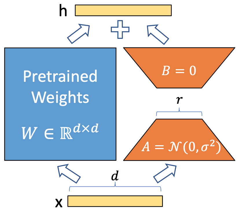
The key idea behind LoRA is that we can model linear projections, that are part of the model's architecture with the product of two smaller matrices. In the transformers architecture such layers are projection matrices that are part of the attention layers (query, key, value and output projections) and projection matrices that are part of the MLP layers.

The Mathematics behind LoRA

LoRA freezes the original weight matrix W of shape \(d\times k\) entirely during the training. Instead, it introduces two small matrices: \(\mathbf{A}\) of shape \(d\times r\) and \(\mathbf{B}\) of shape \(r \times k\), where \(r\) is the chosen rank (usually \(r \ll d, k\). The effective weight during training becomes:

\(\mathbf{W}_{\mathrm{effective}} = \mathbf{W} + \alpha r^{-1}\cdot \mathbf{B} \times \mathbf{A}\)

Here alpha is a scaling hyperparameter, that is usually set to \(2r\). The crucial point is that \(\mathbf{A}\) and \(\mathbf{B}\) together contain only $ r\cdot (d + k)$ parameters instead of \(d \cdot k\). For a projection matrix of size \(4096 \times 4096\), a rank-128 decomposition replaces 16.7 million trainable parameters with just over a million — roughly a 16-times reduction. Only \(\mathbf{A}\) and \(\mathbf{B}\) receive gradient updates; \(\mathbf{W}\) remains frozen. This means we never need to store gradients or optimizer states for the original model weights, slashing the memory requirements dramatically (we still need the W for computing the activations during the forward and backward pass though).

Why does LoRA work? The pre-trained model has already learned a rich representation of language and world knowledge during its initial training on trillions of tokens. Fine-tuning on a domain-specific dataset is asking the model to make relatively targeted adjustments — to shift its prior toward a particular style, vocabulary, or task format — rather than to relearn everything from scratch. Such changes can be modeled using lower-dimension matrices. In addition to compute optimization, LoRA can also help with the downstream task performance, as it limits the catastrophic forgetting (the loss of model's knowledge due to the distribution shift) and may prevent overfitting.

LoRA Configuration

We create the LoRA adapter by passing the LoraConfig from the peft library (PEFT stands for Parameter-Efficient Fine-Tuning) directly to the SFTTrainer:

def use_lora(rank=128):
    # Define LoRA configuration
    lora_config = LoraConfig(
        # task_type=TaskType.CAUSAL_LM,   # Use appropriate task type, e.g., CAUSAL_LM, SEQ_2_SEQ_LM, etc.
        r=rank,  # Rank of the LoRA updates (e.g. 128, 256, 512)
        lora_alpha=2 * rank,  # Scaling factor for LoRA updates (e.g. rank or 2x rank)
        lora_dropout=0.1,  # Optional dropout probability for LoRA layers
        target_modules=[
            "q_proj",
            "v_proj",
            "k_proj",
            "o_proj",
            "gate_proj",
            "up_proj",
            "down_proj",
        ],  # Specify the target modules for LoRA
        bias="none",
        task_type="CAUSAL_LM"
    )

    return lora_config

lora_config = use_lora(rank=lora_rank)

trainer = SFTTrainer(
    ...,
    peft_config=lora_config
)

The most important hyperparameter of the configuration is LoRA rank. The default value (128) sits toward the higher end of what is typically explored. A higher rank gives the adaptation more expressive power, which can be beneficial for more complex tasks. Typically used rank values are 16, 32 and 64. The alpha scaling factor is set to twice the rank, which is a common convention that effectively keeps the magnitude of the LoRA updates in a stable range regardless of what rank is chosen.

Other values that can be set in the LoRA configuration are dropout (we set the dropout probability to 0.1), which serves as light regularisation, target module (list of linear layers, where LoRA is applied), bias and the task type. We apply LoRA to all 7 layer types that appear in the GaMS model and omit the bias. The task type depends on the model architecture. Decoder-type models such as GaMS should be used with the causal language modeling task.

When One GPU is not Enough

DeepSpeed ZeRO Stage 3

Even with LoRA reducing the number of trainable parameters, the frozen base model still needs to reside in GPU memory during the forward pass, and we are training on long sequences (the context is part of the prompt). A single GPU is not enough. To split the model, optimizer and gradients across multiple GPUs, we use DeepSpeed ZeRO (Zero Redundancy Optimizer) Stage 3.

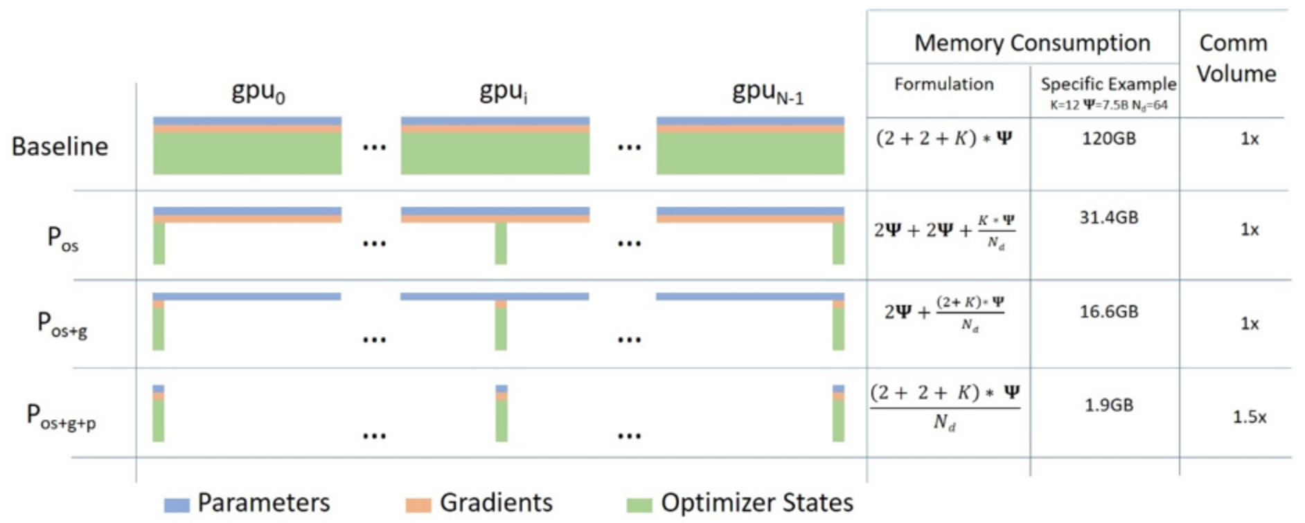
To understand what ZeRO does, it helps to understand the redundancy it is eliminating. In naive data-parallel (each example is put on separate GPU) training, every GPU holds a complete copy of the model weights, gradients, and optimizer states. If the model's optimizer states alone require 100 GB, then across 16 GPUs we are storing 1,600 GB of identical data — 15/16ths of it purely redundant. ZeRO eliminates this redundancy progressively across three stages as visualized on the left.

.

Stage 1 shards the optimizer states: each GPU is responsible for updating only a 1/16th slice of the parameters, so optimizer states are divided by 16. Stage 2 additionally shards the gradients. Stage 3, which we use, goes further and shards the model parameters themselves. At any given moment, each GPU holds only 1/16th of the model's weights. When a layer needs to execute its forward or backward pass, DeepSpeed gathers the relevant parameters from across the cluster, computes through that layer, and then discards the gathered parameters — keeping only the shard that this GPU is responsible for maintaining.

The practical consequence is that very large models can be trained on clusters that could not otherwise fit them at all. The tradeoff is communication overhead: every layer requires an all-gather operation before its computation. The overlap_comm setting in our DeepSpeed configuration instructs the runtime to overlap these communication operations with the computation of other layers wherever possible, hiding much of the latency.

To enable DeepSpeed ZeRO-3 during the SFT training, we define a DeepSpeed configuration in lora_training/deepspeed_config.json. The path to the DeepSpeed config is then passed to the SFTTrainer through SFTConfig. When using ZeRO stage 3 it is essential to define the SFTConfig before initializing the model (using AutoModelForCausalLM.from_pretrained) as the model has to be sharded across GPUs. Additionally, we set device_map=None when loading the model as mapping the model across multiple GPUs is handled by DeepSpeed.

One important detail of the DeepSpeed config is stage3_gather_16bit_weights_on_model_save. Because the model parameters are sharded across GPUs during training, saving a checkpoint naively would produce 16 partial files. This setting instructs DeepSpeed to perform one final all-gather before writing, so each checkpoint is a single complete set of model weights rather than a collection of shards. This makes checkpoints portable and compatible with the merge step that follows training. Many other values in the config are set to auto in order to avoid conflicts, as these values are set in the training script.

Running the job across multiple GPUs

Our training job is structured to run across 4 nodes with 4 GPUs each, giving us 16 GPUs in total.

The Slurm batch script (lora_training/run_sft.sbatch) requests these resources and launches the job using torchrun (since we start multiple processes per node using torchrun, we specify only a single task per node in the Sbatch configuration), which handles the process group initialization that PyTorch's distributed training requires. Each of the 16 processes handles a slice of each training batch, and they communicate gradients and parameter updates via the interconnect between nodes — typically InfiniBand in an HPC cluster (Vega uses InfiniBand), which provides the bandwidth necessary to make multi-node training worthwhile rather than bottlenecked.

Before submitting the job, make sure to set two environment variables in the script. The first is WORK_DIR, which should point to the root directory containing the GitHub repository you cloned. The second is WANDB_API_KEY, that should contain your Weights & Biases API key (discussed further below). Once those are configured, the job is submitted with:

sbatch lora_training/run_sft.sbatch \
    --lora_rank 64 \
    --warmup_steps 500 \
    --learning_rate 2e-5 \
    --min_lr 1e-6

The LoRA rank was already explained. Other three parameters are explained in the sections below.

Learning rate scheduler

The choice of learning rate and how it changes over the course of training is critical to the success of LLM adaptation. Setting the learning rate too high can destabilize the internal representations of the frozen base model, leading to gradient explosion or catastrophic forgetting. Setting it too low results in an inefficient training process that fails to move the model away from its initialization, resulting in poor downstream task performance. To make the training stable, we employ a learning rate scheduler, that changes the learning rate over the time.

We use a cosine decay scheduler with a linear warmup. In the first stage the scheduler linearly increases the learning rate from 0 to the provided learning rate value (keyword argument --learning_rate). This is called a warmup phase and it ensures the model is gently introduced to the new distribution (smaller learning rate at the beginning of the training prevents catastrophical forgetting). The length of the warmup phase is defined by the --warmup_steps parameter. In the second phase, the learning rate is decreased to the minimum learning rate (keyword argument --min_lr) value using the cosine trajectory. The purpose of slowly decaying the learning rate is to make the training more stable in the later steps.

Global and micro batch size and gradient accumulation

Fitting the entire batch of data on single GPU would again cause memory issues. Additionally, when utilizing the multi-GPU training, we want to split the training examples across GPUs (data parallelism). Hence, we differentiate between global batch size and micro batch size (also known as per-device batch size). The first tells on how many examples at once the gradient update is performed (standard batch size in machine learning). The second tells how many examples are simultaneously processed (forward and backward pass) on a GPU. Lower micro batch size results in lower memory consumption. We typically start with micro batch size 1 and then gradually increase it if the hardware permits.

In order to perform a gradient update on a global batch size, we need to accumulate gradients across micro batches. The necessary consequence is that global batch size is divisible by micro batch size. Using the transformers library, the approach is to define the micro batch size and gradient accumulation steps (the number of steps over which the micro batch gradients are accumulated) and the global batch size is computed based on these values. However, in our script, we change this approach and define both batch sizes and manually compute the gradient accumulation steps (defining global and micro batch size is also the standard approach in NVIDIA's training frameworks such as Megatron-LM and NeMo):

# Per-device batch size, adjust based on your hardware
micro_batch_size = 1
# Global batch size
batch_size = 64

world_size = int(os.environ["WORLD_SIZE"])
gradient_accumulation_steps = batch_size // (world_size * micro_batch_size)

We fix the global batch size to 64 examples. Because each GPU processes a micro-batch of 1 example at a time and we have 16 GPUs (this value is obtained from the WORLD_SIZE environment variable, gradient accumulation steps are computed automatically as 64 divided by the total number of GPUs (16), giving 4 accumulation steps per GPU per effective batch. This means each GPU performs 4 forward-backward passes, accumulates the gradients locally, and then synchronises with the other 15 GPUs before the optimizer step. The result is mathematically equivalent to processing all 64 sequences simultaneously on a single enormous GPU, but distributed across the cluster.

Flash Attention 2 and the Memory Cost of Long Sequences

Standard self-attention has a memory cost that grows quadratically with sequence length. For a sequence of \(n\) tokens, the attention matrix has \(n^2\) entries. At the sequence length of 16,384 tokens, that single attention matrix for a single layer requires over 2 GB in bfloat16 — and a GaMS3 has many such layers. This is simply not feasible.

Flash Attention 2 solves this through a restructuring of how the computation is performed. Rather than storing the full \(n \times n\) attention matrix in GPU global memory (the relatively slow high-bandwidth memory, or HBM), Flash Attention 2 tiles the computation: it processes small blocks of the query and key matrices that fit in the GPU's much faster on-chip SRAM, computes a partial attention result, and accumulates the result without ever writing the full matrix to global memory. The final output is mathematically identical to standard attention, but the peak memory footprint for the attention computation is reduced from \(O(n^2)\) to \(O(n)\) in terms of what is held in HBM at any time.

For our use case — long sequences containing a context passage, a question, and a complete answer — Flash Attention 2 is not an optional optimisation. It is what makes training on these sequence lengths possible at all. We enable it by passing attn_implementation="flash_attention_2" to the model initialization.

Liger Kernel and the Cost of Memory Traffic

Modern GPUs are extraordinarily fast at arithmetic but can be surprisingly bottlenecked by memory bandwidth — the speed at which data moves between the GPU's global memory (HBM) and its compute units. Many common neural network operations, such as computing the RMSNorm normalisation used by GaMS3, applying rotary position embeddings (RoPE), or computing the cross-entropy loss, involve multiple sequential GPU kernel launches. Each launch reads data from HBM, performs a relatively small computation, writes the result back to HBM, and then the next kernel reads that result back again. Each round-trip through HBM is time spent waiting.

Liger Kernel addresses this by providing fused implementations of these operations. A fused kernel reads the input once, performs all the constituent operations while the data is still in fast on-chip memory, and writes the final result back to HBM once. For operations like RMSNorm and RoPE that appear in every transformer layer, the cumulative effect on training throughput is meaningful. Liger kernel can increase the training throughput by 20% and reduce memory usage by 60%. We enable Liger Kernel by setting use_liger_kernel=True in the SFTConfig.

Gradient Checkpointing

Every forward pass through the model produces intermediate activations at each layer — tensors that must be retained in memory because they are needed during the backward pass to compute gradients. For a deep model processing long sequences, these activations can collectively consume more memory than the model weights themselves.

Gradient checkpointing (also called activation recomputation) addresses this with a deliberate tradeoff: rather than storing all activations from the forward pass, we store only a selected subset — the "checkpoints" — and recompute the rest during the backward pass when they are needed. The cost is that we perform roughly one additional forward pass's worth of computation per training step. The benefit is a dramatic reduction in peak activation memory, which can be the difference between a batch fitting in memory and running out of it. We enable this by setting gradient_checkpointing=True in the SFTConfig.

Sequence length

Despite all optimisation techniques described above, we might still struggle to fit our training to Vega's 40 GB GPUs (modern AI-optimized clusters have much larger GPUs). Our training data contains some very long examples (extensive context). Another bottleneck is that the gradient checkpointing is not performed during the validation steps, causing peak memory usage during these steps.

To solve this problem, we will limit the maximum sequence length observed during the training and validation to 16,384 tokens. We do this by setting max_length=16384 in the SFTConfig. Using this setting, the SFTTrainer truncates (from the right) all examples that exceed this length. Since we are computing the loss only on completions, this could cause problems for the examples, where the number of prompt tokens exceeds the maximum length. These examples would have all the tokens masked during the loss computation, resulting in NaN loss. To solve this problem, we drop all the examples with too long prompts using the following function:

def remove_long_examples(tokenizer, max_length):
    """
    Removes examples from HF dataset, where prompt exceeds max_length.
    """

    def filter_fn(example):
        prompt_tokens = tokenizer.apply_chat_template(example["prompt"], tokenize=True, add_generation_prompt=True)
        return len(prompt_tokens) < max_length

    return filter_fn

By defining the function that returns boolean values, we can use filter function from the HF datasets.Dataset class. The filter function keeps all examples for which the provided function returns True (examples with prompt tokens below the maximum length in our case) and discards all examples for which the provided function returns False.

Experiment Tracking with Weights & Biases

Training a large model for multiple days without visibility into what is happening is uncomfortable at best and wasteful at worst. Loss curves that diverge, learning rates that are too aggressive, or gradient norms that explode are all problems that are obvious in a training dashboard but invisible if you are simply waiting for the job to finish.

We use Weights & Biases (WandB) to track training runs. WandB is a cloud-based experiment tracking service that records metrics — training loss, validation loss, learning rate, gradient norms — at configurable intervals and makes them available in an interactive browser dashboard in real time. To use it, create a free account at wandb.ai, navigate to your account settings to retrieve your API key, and set it in the SLURM batch script:

export WANDB_API_KEY="your_api_key_here"

The training script passes report_to="wandb" to the trainer through SFTConfig. The logging is handled automatically from that point. Logging frequency is determined by the logging_steps=10 (each 10th step is shown on the WandB graphs) setting of the SFTConfig. If you prefer to run without WandB — for example, when testing on a small subset of data — you can set WANDB_MODE=disabled in the environment, or change report_to to "none". If you are running on a cluster on which compute partition does not have the access to the internet (such example is EuroHPC LEONARDO), you need to uncomment the export WANDB_MODE=offline line in the Sbatch script. In this case all WandB data will be stored only locally and you have to manually synv them with WandB platform from a partition that has the access to the internet.

Checkpointing and Resuming Interrupted Jobs

HPC clusters impose wall-clock time limits on jobs (Vega has the 2-day time limit on the GPU partition). If our training job exceeds that training limit or the cluster experiences an interruption, we need to be able to resume without losing progress.

The SFTTrainer saves checkpoints periodically during training into the output directory, following the naming convention <version>/checkpoint-<step_number>. If a run is interrupted, you can resume it by uncommenting the following line in the run_sft.sbatch script and setting the last checkpoint number:

# TODO: Uncomment and correct the checkpoint number if you are resuming from a checkpoint
# CKPT_PATH=$OUTPUT_DIR/checkpoint-42

The trainer will load the model weights, optimizer states, and scheduler state from the checkpoint and continue training from exactly that step, as if the interruption had not occurred. This makes it practical to run long training jobs on clusters where no single allocation is guaranteed to run uninterrupted to completion.

When the training run finishes, the output directory will contain the LoRA adapter weights — not the full merged model, but the compact A and B matrices that define the adaptation. These adapter weights are small enough to share easily and can either be used directly for inference (vLLM supports loading LoRA adapters at runtime) or merged with the base model weights into a single standalone checkpoint, as described in the following chapter.

Merging the LoRA Adapter into the Base Model

When training completes, the final checkpoint is written to disk. The checkpoint directory does not contain a copy of the full GaMS base model. It contains only the adapter: the two low-rank matrices \(\mathbf{A}\) and \(\mathbf{B}\) for each targeted linear layer, along with the adapter configuration and optimizer state. For a model with billions of parameters, this distinction is profound. Where a full fine-tuned checkpoint might occupy tens or even hundreds of gigabytes, a LoRA adapter trained with rank 64 occupies a small fraction of that space. The frozen base model weights — which constitute the overwhelming majority of the parameter count — were never touched during training, and therefore need not be stored again.

Two Paths to Inference

Once training is complete, there are two natural ways to deploy the result, and understanding their tradeoffs shapes how we think about the merge step.

The first approach is to leave the adapter and base model separate and combine them at runtime. The PEFT library makes this straightforward: load the base model, call PeftModel.from_pretrained with the adapter path, and the combined model is ready for inference. Moreover, libraries such as vLLM let us use multiple different LoRA adapters with the same base model during the inference. This approach is useful when we trained multiple different adapters (either during the hyperparameter search or for different tasks). We can then serve multiple "different" (same base model, different adapter) models while keeping the memory usage low. Additional benefit is that we save storage space.

The second approach is to permanently merge the adapter into the base model weights, producing a single standalone model. This merged model has no dependency on the PEFT library at inference time, behaves exactly like any other transformer, and can be loaded directly by vLLM or any other inference framework without any adapter-specific configuration. There is a modest practical speedup as well, since the matrix addition that would otherwise happen at every forward pass has already been computed once and stored. For production deployment — a single well-validated checkpoint that will serve real users — the merged form is cleaner. Additional benefit is that this approach simplifies another training runs we might perform on top of the specialized model.

Our pipeline focuses on the second approach. In this chapter we describe the merging process.

Performing the Merge

The merge script in merge_lora/merge.py takes four arguments: the path to the base model, the path to the tokenizer (which may differ from the base model path in some configurations - it differs in our case as we combined the tokenizer from the Instruct model, which has chat template, with the base model), the path to the adapter checkpoint, and a name for the output directory where the merged model will be saved.

The checkpoint path follows a consistent convention established by the training script. SFTTrainer saves intermediate and final checkpoints under a subdirectory structure of the form lora_training/experiments/<version>/checkpoint-<step_number>, relative to the training experiments directory. If, for example, training ran for three epochs and saved a checkpoint at step 1500, the adapter path would be something like r-64_ws-500_lr-2e-5_min-lr-1e-6/checkpoint-1500. This naming makes it straightforward to merge from any point in training history, not only the final checkpoint — useful when an evaluation loss suggest overfitting in later steps or we want to test the checkpoints at different steps.

With those paths in hand, the merge proceeds as a short sequence of operations:

# Load the frozen base model in bfloat16
base_model = AutoModelForCausalLM.from_pretrained(
    base_model_path,
    torch_dtype=torch.bfloat16,
    device_map="auto",
)

# Attach the adapter
model = PeftModel.from_pretrained(base_model, adapter_checkpoint_path)

# Fuse adapter weights into base and discard adapter structure
model = model.merge_and_unload()

# Save the merged model and tokenizer as a self-contained artifact
model.save_pretrained(output_path)
tokenizer.save_pretrained(output_path)

The tokenizer is saved alongside the merged weights because any downstream consumer of the merged model — whether an inference server, an evaluation harness, or a colleague — expects to find both in the same directory. Keeping them co-located eliminates one class of configuration error.

To submit the merge job on the cluster, we use the provided Sbatch script, passing the four required arguments:

sbatch merge_lora/run_merge.sbatch \
    cjvt/GaMS3-12B \
    cjvt/GaMS3-12B-Instruct \
    r-64_ws-500_lr-2e-5_min-lr-1e-6/checkpoint-1500 \
    GaMS3-12B-Med

The job will request its single GPU, load the base model, attach and merge the adapter, and write the result to the output directory. Within the 30-minute wall-clock limit, even large models merge comfortably, since the computation is a single pass of matrix additions rather than any form of iterative optimization.

The Mathematics of Merging

The merge operation itself is conceptually simple. During training, each modified weight matrix W in the base model accumulated an update parameterized as the product of two low-rank matrices: a down-projection \(\mathbf{A}\) of shape \((r \times d_{in})\) and an up-projection \(\mathbf{B}\) of shape \((d_{out} \times r)\), scaled by the ratio of the LoRA alpha to the rank \(r\). The effective update to the weight matrix is therefore:

\(\mathbf{W}_{\mathrm{merged}} = \mathbf{W}_{\mathrm{base}} + \alpha r^{-1} \cdot \mathbf{B} \times \mathbf{A}\)

With alpha set to twice the rank in our configuration, the scaling factor simplifies to 2.0, but the PEFT library handles all of this bookkeeping internally. The merge_and_unload() method iterates over every adapted layer, computes this sum, replaces the weight tensor with the merged result, and then discards the adapter matrices entirely. What remains is an ordinary model with no trace of the adapter structure — just slightly different weights than the original base.

The bfloat16 precision used throughout training is preserved during the merge. Loading the base model in bfloat16 before attaching the adapter ensures that the arithmetic happens in the same numerical format as training, and the merged weights are saved in bfloat16 as well. This keeps memory requirements during the merge within reason, which is why the merge job requests only a single GPU with 64 gigabytes of RAM and a 30-minute time limit — a modest allocation compared to the multi-node training run.

Configuration Fix - End of Turn

If we proceeded directly to the inference chapter, we would find out that the trained model does not stop during the inference. The reason for that is the tokenization during the SFT training. During the pretraining, the GaMS model was trained to stop on the end of sequence (EOS) token. However, if we inspect the tokens in the first training example (we printed the first example to the training logs), we would not find token index 1, that corresponds to the EOS token (this is an actual bug in the SFTTrainer tokenization). However, we can spot the token index 106 towards the end of the example. This is the <end_of_turn> token, that GaMS uses to mark the end of each conversation turn (either system, user or assistant). Therefore, the GaMS was trained to produce the <end_of_turn> token at the end of the conversation and we will exploit that by adding this token as EOS token to the model's configuration.

To fix this we will go to the models/GaMS3-12B-Med dir, where the merged model's weights and configurations are stored. We will edit the generation_config.json file that looks like this:

{
  "_from_model_config": true,
  "bos_token_id": 2,
  "eos_token_id": 1,
  "pad_token_id": 0,
  "transformers_version": "4.56.1"
}

We can see that the only EOS token here is 1. We can add the <end_of_turn> token by converting the eos_token_id field to list. Since the <end_of_turn> index is 106, we change the configuration to:

{
  "_from_model_config": true,
  "bos_token_id": 2,
  "eos_token_id": [
    1,
    106
  ],
  "pad_token_id": 0,
  "transformers_version": "4.56.1"
}

Now the model will stop on <end_of_turn> token during the inference. If you check the configuration files on HF repositories of cjvt/GaMS3-12B and cjvt/GaMS3-12B-Instruct, you will observe the exact same difference - the first has only 1 as EOS token, while the second has 106 added as well.

Batch Inference at Scale with vLLM

Once training has finished and the adapter weights are either merged or left intact, the natural next question is how to actually run the model across thousands of examples efficiently. The naive answer — loop over your test set, call model.generate() for each item, wait for the response, move to the next — is conceptually simple but practically disastrous at scale. Each generation call occupies the GPU exclusively while tokens are being produced one at a time, the KV cache for that single sequence is allocated in whatever contiguous memory happened to be available, and the moment that sequence finishes the memory is freed and the next sequence starts from scratch. On a test set of even a few thousand examples, this sequential, memory-fragmented approach can take many hours on hardware that is theoretically capable of far greater throughput. The problem is not compute — it is memory management and the inability to overlap work across requests.

This is the problem that vLLM was built to solve. It enables much faster throughput than transformers library. It enables two types of deployment: offline inference using LLM class, which we show in this service and OpenAI compatible server, that can be reached through API calls (this option is useful when you want to give your customers the access to your model). In this chapter we will show how to implement offline batch inference efficiently. We provide the code in the inference dir. Script vllm_batch_inference.py contains the code for the inference and script run_inference.sbatch contains the Sbatch script to submit the inference job.

PagedAttention and the Memory Management Insight

The key observation behind vLLM is that the KV cache — the stored key and value tensors that the attention mechanism needs to attend over previously generated tokens — does not need to live in a single contiguous block of GPU memory. In traditional inference frameworks, each sequence reserves a large contiguous allocation upfront, sized for the maximum possible sequence length. Most of that reservation goes unused for most sequences, and because the allocations are contiguous, the memory between them cannot be reclaimed for other sequences even when it is technically free. The result is severe memory fragmentation: the GPU has gigabytes of memory that cannot be used productively because it is scattered between reservations.

vLLM borrows a concept from operating systems: virtual memory paging. Just as an OS manages physical RAM by dividing it into fixed-size pages that can be mapped to non-contiguous physical addresses, vLLM manages the KV cache in fixed-size blocks that can be allocated and freed independently. A sequence's KV cache is built up block by block as tokens are generated, and blocks are returned to a global pool the moment they are no longer needed. Crucially, because blocks from different sequences can be interleaved in physical memory, the GPU's memory is used far more efficiently. This technique, called PagedAttention, allows vLLM to keep many more sequences active simultaneously, processing them together in a single batched forward pass. The throughput improvement over naive generation is typically an order of magnitude on longer sequences.

For our purposes, this means that even when individual responses from GaMS can be thousands of tokens long (we allow up to 32,768 output tokens in the inference script), the GPU remains busy processing a full batch throughout the generation process rather than idling between requests.

Batch inference

To run the inference with the vLLM engine, we can directly use the same chat format we used during the training. To recall, we structured our prompt data in the following way:

{
  "prompt": [
    {"role": "system",  "content": "..."},
    {"role": "user",    "content": "..."}
  ]
}

Once we have the data in such format (we perform our inference on test.jsonl, which we already preprocessed a few chapters ago), we can directly call vLLM's model.chat() method on such conversation. The vLLM engine will automatically convert our input to tokens using chat template and produce the output. The output object contains many different fields, that you can check here. In our case, we will extract only the output text.

To additionally speed up our inference, we do not process our examples one by one, but perform inference in batches instead. To do so, we first split our data into batches and then submit the whole batch at once to vLLM by providing the list of requests (each request is a conversation list that is stored under the prompt field in our dataset). The code that handles the batch processing is following:

def process_batch(batch, model, sampling_params):
    prompts = [example["prompt"] for example in batch]
    responses = model.chat(prompts, sampling_params, use_tqdm=False)
    predictions = [response.outputs[0].text for response in responses]

    return predictions

n_batches = ceil(len(dataset) / batch_size)

# Using trange for progress bar
for i in trange(n_batches, desc="Processing Batches"):
    batch = dataset[i * batch_size: min(len(dataset), (i + 1) * batch_size)]
    batch_results = process_batch(
        batch,
        model,
        sampling_params
    )

Tensor Parallelism Across Multiple GPUs

Even with efficient memory management, large language models frequently exceed the memory capacity of a single GPU. GaMS-12B in bfloat16 alone requires roughly 24 GB just for weights, and the KV cache for a batch of long sequences adds substantially more. Our inference nodes provide four GPUs each, and we take advantage of all of them through tensor parallelism. Additional advantage of splitting the model across multiple GPUs is enabling the vLLM engine to process more requests at once as it has more memory available.

The idea behind tensor parallelism is straightforward: the large weight matrices inside each transformer layer are split across multiple GPUs. For a linear layer with a weight matrix of shape [hidden_dim, ffn_dim], we can divide it column-wise across GPUs so that each GPU holds a [hidden_dim, ffn_dim / tp_size] shard. During the forward pass each GPU computes a partial result, and a fast all-reduce communication step (over NVLink in the case of a single node inference) combines these partial results into the full output before moving to the next layer. For the complementary row-parallel layers, the split happens in the other dimension and the partial sums are reduced. For the attention layers the split is also straightforward - each attention layer has multiple attention heads and each attention head can be put on a separate GPU. The net effect is that the model's memory footprint is divided among all participating GPUs, while communication overhead remains small relative to the compute savings.

vLLM handles all of this automatically once we provide the tensor_parallel_size to the LLM initialization call. In our Sbatch script we set the tensor parallel size to $SLURM_GPUS_ON_NODE so the model is split across all GPUs in the node.

Sampling Parameters and Generation Quality

With the model loaded and batching infrastructure in place, we turn to the question of how the model actually generates its responses. Our inference script uses nucleus sampling — also known as top-p sampling — with a temperature of 0.6 and a top-p value of 0.9.

Temperature controls the sharpness of the probability distribution over the vocabulary at each generation step. A temperature of 1.0 leaves the model's raw probabilities unchanged. Values below 1.0 sharpen the distribution, making the model more likely to choose its highest-probability token and less likely to sample surprising alternatives. A temperature of 0.6 sits comfortably in territory that produces focused, coherent text without collapsing entirely into greedy decoding, which can produce repetitive and overly confident outputs.

Top-p sampling adds a second layer of control: rather than sampling from the full vocabulary, we restrict sampling to the smallest set of tokens whose cumulative probability mass reaches 0.9. If the model is highly confident about a single token, that token alone might account for most of the probability mass and sampling is effectively greedy. If the model is genuinely uncertain across many plausible tokens, the nucleus expands to include all of them. This dynamic adjustment of the effective vocabulary size tends to produce text that is both diverse and grammatically coherent.

We set the maximum generation length to 32,768 tokens (this only accounts for completion tokens, the prompt tokens are excluded in this limit). If the model would not stop (by producing EOS or end of turn token) before generating this amount of tokens, the generation will stop at that point (even though the response might be incomplete). However in our case, the answers should be relatively short and 32k tokens should be more than enough.

In code, these parameters are passed as a SamplingParams object to vLLM's model.chat() method, which handles batching and scheduling internally:

from vllm import LLM, SamplingParams

sampling_params = SamplingParams(
    temperature=0.6,
    top_p=0.9,
    max_tokens=32768,
)

model = LLM(model=args.model_path, tensor_parallel_size=args.tp_size)

for batch in batches:
    outputs = model.chat(batch, sampling_params=sampling_params)

SLURM Array Jobs and Dataset Sharding

Processing a full test set on a single node, even with vLLM's throughput advantages, can still take a meaningful amount of time when responses are long and the test set is large. Rather than waiting for a single job to work through thousands of examples sequentially, we distribute the work across eight independent SLURM array jobs that run simultaneously.

A SLURM array job is declared with a single additional flag in the batch script:

#SBATCH --array=0-7

This causes SLURM to launch eight copies of the job simultaneously, each with a different value of $SLURM_ARRAY_TASK_ID ranging from 0 to 7, and with $SLURM_ARRAY_TASK_COUNT set to 8 in each. These two environment variables are passed directly to the inference script as --shard_idx and --n_shards.

Inside the script, sharding is implemented with a single Python slice:

dataset = load_dataset(args.input_file)
shard = dataset[args.shard_idx :: args.n_shards]

This interleaved sharding — where shard 0 takes examples 0, 8, 16, 24, ... and shard 3 takes examples 3, 11, 19, 27, ... — distributes examples evenly across all shards regardless of any variation in example length or difficulty. If we had used contiguous sharding (shard 0 takes the first 12.5% of examples, shard 1 the next 12.5%, and so on), any clustering of long examples in one part of the dataset would cause load imbalance. Interleaved sharding ensures that each shard sees a representative cross-section of the data. However, ordering data by prompt length inside a single shard might be beneficial for the inference throughput - if we did that all the examples in a single batch would be of approximately same length, which could speed up the process.

The practical effect of data sharding is that our total inference time scales nearly linearly with the number of nodes available. Eight nodes complete the job in roughly one-eighth the time of a single node, with no coordination needed between them. Each job is entirely independent: it loads the model, processes its assigned shard, and writes its results to a separate output file.

Fault Tolerance Through Incremental Writing

Long-running HPC jobs are vulnerable to interruption. A node can fail, a power event can occur, or the job can hit its wall-time limit before finishing. If all results are accumulated in memory and written only at the end, an interrupted job loses all of its work. We avoid this by writing and flushing results to disk after every batch:

with open(args.output_file, "a") as f:
    for item, output in zip(batch, outputs):
        result = {**item, "response": output.outputs[0].text}
        f.write(json.dumps(result, ensure_ascii=False) + "\n")
        f.flush()

The flush() call after each write ensures that results reach the filesystem immediately rather than sitting in Python's write buffer. If the job is killed mid-run, every batch that completed before the interruption is safely preserved on disk. Restarting the job from scratch would be wasteful; in practice, one can filter the output file for already-processed example IDs and skip those examples in a re-run.

Each shard writes to its own JSONL file under inference/output/<model_name>/<shard_idx>.jsonl. The original fields from the input dataset are preserved in each output record, with a single additional "response" field containing the model's generated text. This format makes it straightforward to join model outputs back to ground truth for evaluation, and the per-shard files can be processed independently before merging.

Submitting the Inference Job

With all of this machinery in place, launching inference across the full test set reduces to a single command:

sbatch inference/run_inference.sbatch <model_name> <batch_size>

The <model_name> argument identifies both the path from which the model weights are loaded and the subdirectory where output shards will be written, making it easy to keep inference results for different model versions organized. The <batch_size> argument controls how many examples are passed to vLLM's scheduler in a single call; larger batches give the scheduler more flexibility to fill GPU memory efficiently, while smaller batches reduce the peak memory footprint. A batch size of 16 to 32 is a reasonable starting point for sequences of moderate length on four GPUs, though the optimal value depends on the distribution of response lengths in the specific test set being evaluated.

Once all eight array jobs complete, the per-shard JSONL files can be merged into a single unified output file using merge_output.py, after which analyze.py can render the first thirty examples in human-readable form for a quick sanity check on generation quality before proceeding to quantitative evaluation. We describe this in the next chapter.

Prediction Analysis

The inference stage leaves us with eight independent JSONL files scattered across a subdirectory — one per array job task, each containing roughly one-eighth of the test set's predictions. Before we can draw any conclusions about our fine-tuned model's capabilities, these fragments need to be reassembled into a coherent whole, and more importantly, we need to actually read what the model produced. This chapter covers both of those steps: the mechanical work of merging sharded output, and the intellectually irreplaceable practice of qualitative inspection.

Reassembling the Shards

The sharded output is a direct consequence of the array job design we chose for inference. Each SLURM task processed its own slice of the test set independently, writing results to its own file under inference/output/<model_name>/. The path looks something like this after a completed inference run:

inference/output/GaMS3-12B-Med/
    0.jsonl
    1.jsonl
    2.jsonl
    ...
    7.jsonl

There is nothing wrong with this structure during inference — it is precisely what made the parallelism possible — but it is inconvenient for everything that comes after. Evaluation frameworks, human review tooling, and downstream pipelines all expect a single file. The merge_output.py script handles this consolidation. It collects every .jsonl file it finds in a given directory and concatenates their contents into a single output file:

python inference/merge_output.py \
    --input_dir inference/output/GaMS3-12B-Med \
    --output_file inference/output/GaMS3-12B-Med_merged.jsonl

The implementation is simple: it scans the input directory for files ending in .jsonl, reads them line by line, and writes each parsed record to the output. This simplicity is a feature rather than a limitation, but it comes with one caveat worth internalising: shard order is not guaranteed. The eight tasks ran concurrently on independent nodes, and the files may be concatenated in filesystem-dependent order. If your downstream evaluation requires predictions to be in a consistent sequence — for instance, if you are aligning predictions against a gold reference file by line number — you should sort the merged records by their id field before passing them on.

Conversion to human readable format

There is a temptation, especially in a pipeline as automated as this one, to go directly from merged predictions to quantitative metrics. BLEU scores, ROUGE-L, BERTScore, or an LLM-as-judge setup can all be computed in minutes and produce satisfying-looking numbers. The problem is that automated metrics are optimized to summarize a distribution, and in doing so they can average over catastrophic failures that affect every single example.

The analyze.py script is designed for exactly this purpose. It takes the merged predictions file and produces a human-readable text document containing the first thirty examples from the dataset. For each example, it renders the full prompt — system message, user turn, and context if present — followed by a clear delimiter and the model's complete response. Running it is straightforward:

python inference/analyze.py \
    --input_path inference/output/GaMS3-12B-Med_merged.jsonl \
    --output_path inference/output/GaMS3-12B-Med_analysis.txt

The output file is meant to be read slowly, not skimmed. Thirty examples is a deliberately small number; the goal is depth of attention, not breadth of coverage. When reading through the analysis file, there are several dimensions worth evaluating deliberately. First, language consistency: is every response in Slovenian, and is the language fluent? Second, answer completeness: does the model actually answer the question asked, or does it hedge, deflect, or repeat the question back in different words? Third, context fidelity for the examples that include a retrieved passage: does the model's answer draw on the provided context, or does it ignore it in favour of its parametric knowledge? Fourth, factual plausibility. Are there answers that are internally inconsistent, implausibly confident about obscure specifics, or that contradict information stated explicitly in the prompt.

The thirty-example window will not catch every failure mode in a test set of several hundred examples, but it reliably surfaces systematic problems. If the model is doing something wrong, it is usually doing it consistently, and that consistency will be visible within the first page or two of the analysis file.