Samodejno generiranje prometnih poročil

Pregled

Produkcijski sistem, ki nacionalni prometni vir podatkov pretvarja v poročila, pripravljena za radijsko objavo. Storitev fetcher redno zajema dogodke, dela na cesti in uradna prometna poročila iz vira NAP, iz njih odstrani podvojene zapise in jih normalizira v enotno strukturo v zbirki PostgreSQL. Lokalno dodatno naučen klasifikator ModernBERT nato vsakemu dogodku določi nujnost glede na uredniška merila, zapisana skupaj z uredniki RTV Slovenija, tako da časovno kritični primeri, na primer prometne nesreče, vozniki v napačno smer in popolne zapore, ne čakajo na naslednje redno poročilo. Izbrani zapisi gredo skozi dvostopenjski cevovod generiranja; prva stopnja iz vsakega zapisa izlušči strukturirane pomenske enote, druga pa jih razvrsti in sestavi v slovenščino, posebej prilagojeno za radijsko poročanje. Obe stopnji uporabljata enotno obliko zahteve, zato lahko isti klic obdela bodisi lokalno gostovan in dodatno naučen model GaMS3-12B-Instruct bodisi OpenAI API, s samodejnim preklopom med njima. Uredniki vsako poročilo pregledajo, uredijo ali zavrnejo v aplikaciji Angular, ki nova poročila in nujna opozorila prejema v realnem času prek povezave WebSocket.

Rezultat

Uredniki v nekaj sekundah po pojavu dogodka v viru prejmejo osnutke prometnih poročil v slovenščini, pripravljene za objavo, pri čemer nujni dogodki prehitijo redni cikel. Vsak generiran stavek ostaja sledljiv do zapisov NAP, iz katerih je nastal, končno odločitev pa ohranijo uredniki, saj brez človeške potrditve nič ne gre v objavo. Uredniški popravki in povratne informacije se shranjujejo kot strukturirani zapisi, kar gradi vse obsežnejšo zbirko za vrednotenje in izboljševanje klasifikatorja nujnosti ter pozivov za generiranje.

Kartica storitve

Kategorija	AI products
Domena	Generiranje naravnega jezika, prometne informacije, radijsko poročanje
Vertikala	Mediji in novinarstvo
Ciljni uporabniki	Medijske organizacije in uredništva, podjetja in raziskovalne skupine s področja umetne inteligence ter vse organizacije, ki morajo strukturirane podatke velikega obsega pretvarjati v ponavljajoča se poročila v naravnem jeziku
Tip storitve	Cevovod, Model, Aplikacija
Nosilec	Univerza v Ljubljani, Fakulteta za računalništvo in informatiko (v sodelovanju z RTV Slovenija)
Rezultat	Prometna poročila v slovenščini, pripravljena za radijsko objavo; razvrstitev nujnosti za vsak dogodek s popolnim dnevnikom vseh odločitev; povezave za sledljivost vsakega poročila nazaj do izvornih zapisov; strukturirani zapisi uredniških povratnih informacij; zabeleženi klici modelov z navedbo ponudnika za analizo stroškov in kakovosti; celoten sklad kot storitve Docker z nadzorom Prometheus in Grafana.
Zahteve	Dostopni podatki za strukturiran prometni vir, v referenčni namestitvi je to vir NAP B2B. Gostitelj Docker za priložene storitve, torej zaledni del Flask, PostgreSQL, Redis, vmesnik Angular in Traefik. Ključ API oblačnega ponudnika jezikovnih modelov, če se uporablja oblačna pot, ali končna točka, združljiva z OpenAI Responses API, če je model gostovan lokalno, pri čemer je za lokalno gostovanje dodatno naučenega modela priporočljivo vozlišče z grafično kartico.
Omejitve	Izhod je trenutno v slovenščini, čeprav je prilagoditev pozivov za generiranje na drug jezik razmeroma hitra. Zajemni del je napisan za shemo vira NAP, klasifikator nujnosti pa vsebuje en določen nabor uredniških pravil natanko tako, kot so bila zapisana, zato uporaba sistema na drugem viru ali z drugačno opredelitvijo nujnega dogodka zahteva preslikavo izvornih polj in ponovno učenje klasifikatorja na novih pravilih. Kakovost generiranja je odvisna od popolnosti vhodnih zapisov, lokalno gostovan model pa po tekočnosti še nekoliko zaostaja za oblačnim.
Na voljo	V produkcijski uporabi na RTV Slovenija
Licenca	Podatki so odprto dostopni, saj je nacionalni prometni vir NAP javen. Aplikacija sama je zasebna in lastniška, sistem za generiranje poročil ni objavljen pod odprto licenco.

Uvod

Priprava prometnega poročila za radijsko objavo je bila doslej ročno uredniško opravilo. Urednik primerja več prometnih virov, iz rutinskih dogodkov izlušči tiste, ki so pomembni, združi poročila o istem dogodku in rezultat prepiše v kratke, za branje primerne slovenske povedi — pod pravim časovnim pritiskom, saj morajo nujni dogodki, na primer prometne nesreče ali vozniki v napačno smer, do poslušalcev priti v nekaj minutah in ne šele ob naslednjem rednem poročilu. Postopek je zamuden in po naravi subjektiven: dva urednika lahko iz istega vira izbereta različen nabor »pomembnih« dogodkov, kakovost končnega poročila pa je močno odvisna od posameznikove presoje in razpoložljivega časa.

Veliki jezikovni modeli so naravna izbira za pretvarjanje strukturiranih podatkov velikega obsega v naravni jezik: povezane dogodke združujejo, prilagajajo ton in besedilo krajšajo precej hitreje kot urednik, ki dela sam. Vendar zgolj usmeritev splošnonamenskega modela na surov prometni vir za produkcijsko uredništvo ne zadošča. Prometni zapisi vsebujejo veliko odvečnih podatkov, se ponavljajo in niso enotno oblikovani; model, ki jih prosto pripoveduje, si lahko izmisli podrobnosti, ki jih v viru ni bilo, tiho izgubi povezavo z zapisom, ki ga je povzel, in se ob vsaki spremembi poziva vsebinsko premakne — kar pri radijskem poročanju, kjer mora biti vsaka izgovorjena poved sledljiva in kjer mora končno besedo ohraniti urednik, ni sprejemljivo.

Ta delovni tok opisuje sistem, zgrajen za reševanje tega problema na RTV Slovenija: kako se prometni podatki zbirajo in pripravljajo, kako se nujni dogodki ločijo od rutinskih, kako dvostopenjski cevovod generiranja iz strukturiranih zapisov ustvari besedilo, primerno za radijsko objavo, in kako je bil lokalno dodatno naučen odprti model zgrajen ter primerjan z oblačnim, da bi zmanjšali stroške in zunanjo odvisnost. Sistem je v aktivni produkcijski uporabi; ta delovni tok ne pojasnjuje le, da deluje, temveč tudi, zakaj je bila vsaka zasnovna odločitev sprejeta tako, kot je bila, da je mogoče iste odločitve pretehtati pri gradnji podobnega sistema drugje.

Sorodni pristopi

Pretvarjanje strukturiranih virov v kratka, objavljena besedila ima uveljavljeno produkcijsko zgodovino, ki je starejša od velikih jezikovnih modelov. Poročila o dobičkih agencije Associated Press (zgrajena s Automated Insights) in Heliograf časnika The Washington Post sta pokazala, da se generiranje besedila iz podatkov dobro obnese, kadar je osnovna naloga ponavljajoča se in jasno strukturirana, sistema Quakebot časnika Los Angeles Times ter Tracer in Lynx Insight agencije Reuters pa sta vzorec razširila z zaznavanjem dogodkov in filtriranjem pomembnosti pred pisanjem — vedno tako, da je urednik ostal zadnja stopnja pred objavo. Bliže domeni tega projekta sta sodelovanje družbe Bauer Media s Fintraffic in INRIX-ov AI Traffic Reporter, ki sta na več trgih že uvedla lokalizirana prometna poročila, generirana z umetno inteligenco. Ta projekt od njih ločuje kombinacija izhoda v slovenščini, nacionalnega prometnega vira NAP kot edinega vira resnice, izrecne sledljivosti vsake generirane povedi nazaj do izvornega zapisa in premišljene zasnove, ki urednika ohranja v zanki, namesto da bi ga nadomestila.

Sistem na kratko

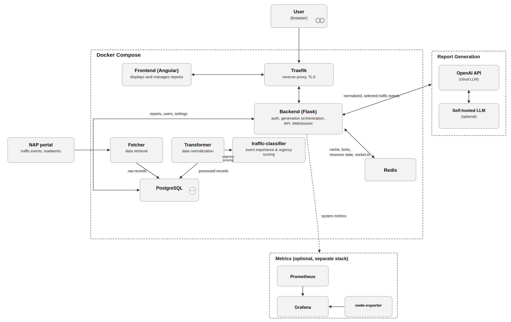
Cevovod, ki ga ta delovni tok obravnava, sestavljajo štirje gradniki. Podatkovni cevovod (fetcher in transformer) redno zajema prometne dogodke, dela na cesti in poročila iz vira NAP, iz njih odstrani podvojene zapise in jih normalizira v enotno strukturo, shranjeno v zbirki PostgreSQL. Klasifikator nujnosti (traffic-classifier), lokalno dodatno naučen kodirni model, oceni vsak normaliziran dogodek, tako da je časovno kritične primere mogoče usmeriti pred rutinske. Dvostopenjsko generiranje, ki ga vodi backend, iz izbranih zapisov najprej izlušči strukturirane pomenske enote, nato pa jih sestavi v slovensko besedilo, posebej prilagojeno za radijsko poročanje, pri čemer glede na nastavitve in razpoložljivost samodejno preklaplja med lokalno gostovanim modelom in OpenAI API. Nazadnje aplikacija za urednike (vmesnik Angular frontend) v realnem času prek povezave WebSocket prikazuje generirana poročila, izvorne zapise in nujna opozorila ter urednikom omogoča, da poročilo pred objavo uredijo, potrdijo ali zavrnejo.

Vsebina delovnega toka

Poglavja, ki sledijo, cevovod spremljajo od podatkov do namestitve, vsako pa je zamejeno dovolj ozko, da ga je mogoče brati samostojno, če ste s posameznim delom že seznanjeni. Začnemo pri podatkih samih: Podatkovni viri obravnavajo živi vir NAP ter cevovod zajema, shranjevanja in normalizacije za njim, Ujemanje z zgodovinskimi poročili pa pojasnjuje, kako so bili arhivski prometni zapisi iz Excela ujemani z arhivskimi radijskimi poročili (z uporabo TF-IDF in kosinusne podobnosti), da so nastali pari za vrednotenje in učenje, na katerih temelji vse nadaljnje.

Od tod preidemo k modeloma, ki ju ta delovni tok neposredno primerja. Klasifikacija dogodkov celovito obravnava klasifikator nujnosti — njegove atribute in uredniška pravila, zgrajena nanje, kako so bili učni podatki označeni in uravnoteženi ter kakšen dvofazni učni načrt je bil uporabljen. Inženiring pozivov obravnava zasnovo dvostopenjskega generiranja, Generiranje poročil pa to, kdo jo dejansko izvede, kakšno vlogo imata oblačni in lokalni model v istem cevovodu, kako deluje preklop med ponudnikoma in kaj produkcija zares beleži, medtem ko Lokalni model za generiranje dokumentira, kako je bil lokalno gostovani model GaMS3-12B-Instruct dodatno naučen in kvantiziran, da služi kot cenejša alternativa. Primerjava in vrednotenje modelov obe poti postavi drugo ob drugo glede kakovosti, stroškov, prilagodljivosti na spremenjen poziv, ravnanja s podatki in vzdrževanja.

Zadnje poglavje obravnava sistem, kakršen v resnici teče: Arhitektura aplikacije predstavi nameščene storitve, razloge za njihovo razdelitev in uredniški postopek pregleda.

Data Sources

The quality of a generated traffic report is bounded by the quality, freshness, and structure of the data that goes into it. No amount of prompt engineering compensates for a report built on stale, duplicated, or ambiguous input. The system therefore draws on two distinct data sources, used for two different purposes. Historical data, archived Excel traffic records paired with archived RTF radio bulletins, was used only during development, to understand the editorial process and build training and evaluation examples. Live data from the national NAP access points is what the production system actually runs on. This chapter describes both, and, just as importantly, how the two were reconciled, since a model built or tested on historical data is only useful if it later receives comparable input in production.

Historical Data

Historical data served four purposes during development: understanding the structure of traffic information as editors work with it, analyzing how editors select and phrase reports, testing different generation approaches before committing to one, and preparing the training and evaluation examples used throughout this workflow. Two sources made this possible.

Archived Excel Traffic Records

The archival traffic records arrived as Excel files, one row per timestamped snapshot. Each row's text fields contained HTML-formatted content split into several topical sections:

Field	Meaning
LegacyId	Unique identifier of the record in the archival export
Datum	Timestamp of creation or last update
Operater	The person or source who authored or edited the record
Pomembno	Highlighted, urgent traffic information
Nesreče	Accidents and their impact on traffic
Vreme	Weather-related traffic conditions
Ovire	Obstacles on the road or other disruptions
DeloNaCesti	Roadworks, closures, and altered traffic arrangements
Opozorila	General warnings, forecasts, restrictions, and other notices
MednarodneInformacije	Information related to border crossings or international traffic
Zastoji	Congestion, tailbacks, and longer travel times
Splošno	General traffic information not tied to a single concrete event

A single row can contain several topical sections and several distinct events at once, so the number of rows is not the number of unique traffic events. Across the three years available, the archive holds:

Period	Records	Avg. records/day
2022	55,001	150.7
2023	57,094	156.4
2024	58,278	159.2
Total	170,373	155.4

Archived Radio Reports

Alongside the Excel records, an archive of radio traffic bulletins was available as RTF files. These represent the target form of the output: they show how editors, working from a much larger pool of raw traffic information, chose the handful of events worth reporting and rewrote them into short, speaker-ready Slovenian. Because the two archives were not linked by a shared identifier, building usable pairs between "what was available" and "what was actually broadcast" required a dedicated matching procedure, covered in the next chapter, Historical Report Matching.

Comparing the two archives directly was itself informative: source records are consistently longer, more technical, and denser in detail, while radio reports require selecting only the most important events, shortening aggressively, merging related events, and adapting the language to a spoken medium. This gap between "raw input" and "broadcast output" is precisely what later motivated a structured, two-stage generation approach rather than asking a model to write directly from raw records — see Prompt Engineering.

Live Data from NAP Access Points

In production, the system no longer reads from Excel exports — it polls the national traffic data portal, NAP, directly. NAP technically exposes three access points: traffic events, roadworks, and traffic reports. Of these, traffic events and roadworks are the two that matter for generating radio bulletins, since they contain individual, current records of road conditions. The traffic reports access point is also fetched and stored, but mainly for archival and comparative analysis rather than as direct generation input.

Unlike the archival Excel rows, records from NAP are already structured as discrete events rather than free-flowing text. A typical record carries a unique identifier, an update timestamp, the affected road or road segment, a road category, a cause (vzrok), a description of the conditions, and an optional additional explanation. Because these are structured events rather than prose, they can be stored, compared, deduplicated, and ranked programmatically — which is exactly what the ingestion pipeline (the fetcher and transformer services) does before any record reaches a language model.

Access to NAP is authenticated with OAuth2: the fetcher acquires an access token with a username and password, then renews it with a refresh token before expiry, proactively, ahead of time, and reactively, if a request ever comes back with a 401. Each of the three access points is polled independently, on its own configurable interval, and every request is conditional: if the source reports that nothing has changed since the last poll, no rows are rewritten. The system simply advances a "still present" timestamp on the previously seen records. This distinction matters downstream: it lets the pipeline tell "this event hasn't changed since last time" apart from "this event is no longer being reported by the source," which in turn drives both staleness filtering and the freshness checks applied before generating a report (see Prompt Engineering).

Reconciling Historical and Live Data

A model tuned or evaluated on historical Excel data is only as useful as its similarity to what the production system will actually feed it. This mattered because the two sources don't describe traffic information the same way: the Excel archive organizes content into topical sections, while NAP structures it around a single vzrok (cause) field. Before historical data could be used to build comparable inputs, each Excel content section had to be checked against the values that actually appear in NAP's vzrok field:

Historical section (Excel)	NAP vzrok value	Comparability
Delo na cesti (roadworks)	Delo	Comparable
Zastoji (congestion)	Zastoj	Comparable
Ovire (obstacles)	Ovire	Comparable
Nesreče (accidents)	Nesreča	Comparable
Vreme (weather)	Vreme	Comparable
Omejitve za tovorna vozila (truck restrictions)	Tovornjaki	Comparable
Pomembno (highlighted/urgent)	Vožnja v nasprotno smer (wrong-way driving)	Partially comparable
Splošno (general)	(none)	Not comparable
Mednarodne informacije (international)	(none)	Not comparable
Opozorila (warnings)	(none)	Not comparable

Six sections mapped cleanly and became the main basis for building comparable historical inputs: roadworks, congestion, obstacles, accidents, weather, and truck restrictions. The Pomembno section was only partially usable — it bundles several safety-critical situations (wrong-way driving being the clearest example) that NAP instead represents as ordinary vzrok values in their own right, so entries had to be reinterpreted rather than mapped one-to-one. The remaining three sections had no counterpart in NAP at all and were excluded from data used to build or evaluate models, since a model trained on them would learn to expect input the production feed simply never provides.

This distinction (comparable, partially comparable, not comparable) also anticipated a second problem: NAP does not flag any event as "urgent." A traffic accident, a long tailback, or a wrong-way driver arrives in the feed looking like any other record. Telling these apart from routine events at the speed radio broadcasting requires is the job of the classifier described in the next data-facing chapter, Event Classification.

Historical Report Matching

The two historical archives described in the previous chapter (raw Excel traffic records and archived RTF radio bulletins) were never linked by a shared identifier. An editor who wrote a bulletin at 20:00 did not record which specific traffic records they used to write it. Turning these two archives into usable training and evaluation examples, pairs of "what the system would have seen" and "what should have been broadcast", required an approximate matching procedure. This chapter walks through that procedure as it was actually implemented, with the real code behind it.

Reusable Pattern

When two datasets should correspond but aren't linked by a shared key, and both sides describe the same underlying events in overlapping language, e.g. an archived report and the raw records it was likely written from, sharing road names, causes, and similar phrasing, a bounded time window plus TF-IDF and cosine similarity is a fast, low-dependency way to build approximate pairs worth training or evaluating on.

Preparing Both Sides

Before any matching can happen, both archives need to be in a comparable, structured form.

The Excel records store their content as an HTML blob per row, with each <strong> tag marking a topical heading (Nesreče, Delo na cesti, and so on, as described in Data Sources) followed by its text. A small parser turns each row into a plain dictionary keyed by heading:

from bs4 import BeautifulSoup

def parse_html_to_dict(html_text: str) -> dict:
    """Parse an HTML block into {heading: text}, using each <strong> tag as a key."""
    if not html_text:
        return {}

    soup = BeautifulSoup(html_text, "html.parser")
    for br in soup.find_all("br"):
        br.replace_with("\n")

    result, current_key, buffer = {}, None, []
    for p in soup.find_all("p"):
        strong_tags = p.find_all("strong", recursive=False)
        text_outside_strong = "".join(p.find_all(text=True, recursive=False)).strip()

        if len(strong_tags) == 1 and not text_outside_strong:
            if current_key and buffer:
                result[current_key] = " ".join(buffer).strip()
                buffer = []
            current_key = strong_tags[0].get_text(strip=True)
        else:
            text = p.get_text(" ", strip=True)
            if text:
                buffer.append(text)

    if current_key and buffer:
        result[current_key] = " ".join(buffer).strip()
    return result

Each row is then reduced to its LegacyId, Datum, Operater, and this parsed content dictionary, and the whole sheet is written out as JSON (one file per year) so the rest of the pipeline never has to deal with Excel or raw HTML again.

The RTF bulletins need the opposite treatment: extracting structure out of what is otherwise a wall of text. Each file is converted to plain text, split into blocks, and its first line is parsed as a header containing a title, date, time, and programme:

import re
from striprtf.striprtf import rtf_to_text

date_pattern = re.compile(r"\b\d{1,2}\.\s?\d{1,2}\.\s?\d{4}\b")
time_pattern = re.compile(r"\b\d{1,2}[:.]\d{2}\b")

def parse_header(line):
    date_match, time_match = date_pattern.search(line), time_pattern.search(line)
    date = date_match.group().replace(" ", "")
    time = time_match.group().replace(",", ".")
    title = line[:date_match.start()].strip()
    programme = line[time_match.end():].strip()
    return title, date, time, programme

Headers that don't contain a parseable date and time are flagged and dropped — a small number of archived files had corrupted or non-standard headers, and it is safer to discard them than to guess. Everything after the header becomes the report's content.

Finding Candidate Matches

A radio bulletin can only have been written from traffic records that already existed by the time it aired. For each report, the matching procedure first narrows the field to Excel records created within a fixed time window before the bulletin's timestamp — three hours proved to be a reasonable compromise between recall and search cost:

from datetime import datetime, timedelta

def parse_report_dt(r):
    return datetime.strptime(f"{r['dan'].strip()} {r['čas'].strip().replace('.', ':')}", "%d.%m.%Y %H:%M")

def parse_excel_dt(e):
    return datetime.strptime(e["Datum"], "%Y-%m-%d %H:%M:%S")

def find_prior_excel_entries(report_row, excel_data, hours=3):
    r_dt = parse_report_dt(report_row)
    window_start = r_dt - timedelta(hours=hours)
    matches = [(parse_excel_dt(e), e) for e in excel_data if parse_excel_dt(e)]
    matches = [(dt, e) for dt, e in matches if window_start <= dt <= r_dt]
    matches.sort(key=lambda t: t[0], reverse=True)
    return matches

This step alone typically narrows thousands of yearly records down to a short list of candidates per report — small enough to rank by actual text similarity.

Ranking Candidates by Text Similarity

Within that short list, the report and every candidate record are cleaned the same way: lowercased, stripped of control characters, and reduced to their non-stopword, non-punctuation lemmas using a Slovenian spaCy model, before being compared:

import spacy
from sklearn.feature_extraction.text import TfidfVectorizer
from sklearn.metrics.pairwise import cosine_similarity

nlp = spacy.load("sl_core_news_sm")

def clean_text(text: str) -> str:
    text = re.sub(r"[\x00-\x1F\x7F]", " ", text).lower()
    tokens = [t.text for t in nlp(text) if not t.is_stop and not t.is_punct and not t.is_space]
    return " ".join(tokens)

# report_sample: the radio bulletin; matches: candidates from find_prior_excel_entries
cleaned_content = clean_text(report_sample["content"])
cleaned_matches = [clean_text(str(m[1]["content"])) for m in matches]

corpus = [cleaned_content] + cleaned_matches
tfidf = TfidfVectorizer(min_df=1).fit_transform(corpus)
similarities = cosine_similarity(tfidf[0], tfidf[1:]).flatten()

top_3 = similarities.argsort()[::-1][:3]

Fitting a fresh TF-IDF vectorizer per report (rather than one global vocabulary) keeps each comparison local to the handful of candidates that could plausibly be the source, which matters because the vocabulary of a three-hour slice of traffic records is small and topic-specific. The top three candidates by cosine similarity are kept for every report, together with their similarity score, so that low-confidence matches remain inspectable rather than silently discarded.

Selecting the Best Matches

Each report already had its top three candidates from the ranking step above. To turn that into a final corpus, only the single best-scoring candidate per report was kept, and reports were then sorted by that score, highest-confidence first; the 100 top-scoring pairs per year became the matched corpus:

all_best = []
for report in report_matches:
    report["best_match"] = max(report["top_matches"], key=lambda x: x["score"])
    all_best.append(report)

all_best.sort(key=lambda x: x["best_match"]["score"], reverse=True)
top_100 = all_best[:100]

An example

One of the strongest matches from 2023 illustrates what a good pair looks like. The broadcast bulletin read:

Nujna prometna informacija: Predor Karavanke je zaradi izrednega prevoza zaprt proti Avstriji. ("Urgent traffic information: the Karavanke tunnel is closed toward Austria due to an oversized transport.")

The score (0.65) isn't computed against one relevant line picked out of the Excel row; it's computed against the row's whole content dict, every heading it carries, stringified together (that's the str(m[1]["content"]) in the ranking step above, not a per-heading comparison). This particular row's dict happens to hold only one heading, Pozor! ("Attention!"), so the whole row and the text below are one and the same — a row with several headings would have had all of them contribute to the score, not just the one that turned out relevant:

Predor Karavanke je zaprt proti Avstriji zaradi izrednega prevoza.

The two sentences are near-identical after cleaning — exactly the kind of pair that confirms the matching procedure is finding genuine source-to-broadcast correspondences rather than coincidental overlap. It's also a reminder from the previous chapter's dedup discussion: this record appeared under three consecutive LegacyIds with identical content, since NAP-style sources re-confirm unchanged events across snapshots rather than emitting them once.

Why This Matters, and What's Next

These matched pairs became the backbone of several later chapters: they're the training and evaluation examples used to compare generation approaches (see Model Comparison & Evaluation), and a source of labeled examples for the urgency classifier (see Event Classification).

The approach is deliberately simple. A more sophisticated matching method, one that understood paraphrase or could align partial, merged events, would have taken more time and research than this project had available, so TF-IDF and a time window were chosen as the fastest path to a corpus that was good enough to build on. That tradeoff comes with a few weaknesses worth naming rather than glossing over. The three-hour window is a heuristic: it works well for events reported close to when they were first recorded, but it can miss cases where the underlying record (a long-running roadwork, for instance) is genuinely older than the window allows. TF-IDF and cosine similarity reward near-verbatim overlap, so they excel at exactly the kind of case shown above, but score lower on reports where an editor paraphrased heavily, merged several distinct events into one sentence, or added context that wasn't in any single source record. In practice, this means match scores are a confidence signal, not a guarantee, which is exactly why the corpus was built from the top of that ranking rather than from every candidate pair a report happened to produce.

Event Classification

NAP does not tell you which events matter. A wrong-way driver, a full road closure, and a pothole notice all arrive in the feed looking like ordinary records: same shape, same fields, no urgency flag. So far, it was on RTV Slovenija's editors to make a judgement whether an event is urgent or not and treat it accordingly, but before any of that editorial judgment could be automated, it first had to be made explicit, written down as criteria a machine could check, and built into a model and a dataset that could learn them.

This chapter follows that path in the order it was actually built: what a raw event looks like before any classification happens, what new information gets added on top of it, how that information was labeled and balanced into a trainable dataset, how the model itself was trained, and how its predictions are actually turned into an urgent/not-urgent verdict.

Reusable Pattern

Predicting several interpretable sub-attributes and deriving a final verdict from them with explicit rules, rather than training a model to output one opaque label directly, keeps the classifier's behavior auditable and easy to adjust without retraining. For this kind of short-text, structured multi-attribute classification, a small shared encoder with several task-specific heads on top is usually a better fit than reaching for a large language model: faster and cheaper to run per event, and trainable on a comparatively modest labeled dataset.

Classifier Training Data

The Raw Event: Cause and Description

Before any classification, a NAP event is just a handful of fields — a road, a category code, and two pieces of free text:

{
    "kategorija": "A2",
    "cesta": "A2-E70, Obrežje - Ljubljana",
    "vzrok": "Okvara vozila",
    "opis": "A2, Obrežje - Ljubljana, priključek Višnja Gora - priključek Grosuplje vzhod v smeri Ljubljane, okvara vozila, zaprt prehitevalni pas.",
    "dodatno_pojasnilo": ""
}

vzrok (cause) is the closest thing to a category NAP gives you, with values like Nesreča, Zastoj, Delo, Okvara vozila. opis is a free-text description written for a human reading the source portal, not for a downstream system. Neither field says whether this particular breakdown, on this particular road, is worth interrupting programming for. That judgment has to come from somewhere else.

The Ten Attributes We Add

On top of every raw event, the system adds ten pieces of structure that don't exist in the NAP feed at all: nine independent yes/no attributes, and one five-way classification of the road itself.

Attribute (API)	Model head (Slovenian)	What it captures
wrong_way_driving	Vožnja v napačno smer	Vehicle traveling against the direction of traffic
accident_lane_closure	Nesreča - zapora pasu	Accident that has closed one or more lanes
accident_full_closure	Nesreča - popolna zapora	Accident that has closed the road entirely
road_lane_closed	Cesta/pas zaprt	Any road or lane closure, regardless of cause
object_on_road	Ovira na cesti	An obstacle or debris on the roadway
major_congestion	Velika gneča (≥30min)	Congestion adding 30+ minutes of travel time
emergency	Nujnost	General emergency indicator
safety_risk	Varnostno tveganje	Explicit danger to drivers
scheduled_event	Načrtovan dogodek	Planned rather than incident-driven (e.g. a scheduled closure)

Tip ceste (road type) classes
Avtocesta (motorway) · Hitra cesta (expressway) · Glavna cesta (main road) · Regionalna cesta (regional road) · Občinska cesta (municipal road)

These ten values are what the classifier is actually trained to predict from opis — everything from here on is about how that training happened. What they're used for, once predicted, is covered at the end of this chapter.

Labeling Real Events with GPT-5.2

Training all ten heads at once required a dataset labeled on all ten at once. 14,508 real historical events were labeled attribute by attribute using GPT-5.2 as a one-time labeling tool — not the production classifier itself, just a way to bootstrap ground truth. Hand-labeling that many events across ten attributes was never realistic, and a large general-purpose model's judgment, applied consistently across the whole set, was a practical substitute for it. This is the same kind of role a cloud LLM plays elsewhere in the system: not the thing running at request time, but the thing that made a smaller, faster, purpose-built model possible in the first place (see Report Generation for where GPT plays a very different, production-facing role instead).

The Class Imbalance Problem

Real traffic events are heavily skewed toward the routine. Of the 14,508 GPT-labeled events, wrong-way driving appears in just 30 (barely a fifth of a percent), and major congestion and scheduled events are almost as rare, at 144 and 354. A handful of attributes sit at the other extreme: safety_risk and emergency each appear in nearly half the data. A head trained directly on wrong_way_driving at that ratio has an easy way to minimize loss: always predict "no," and be right 99.8% of the time while being useless in exactly the cases that matter.

Road type has its own, different kind of imbalance: of the original events, 10,212 are on an Avtocesta against just 108 on an Občinska cesta — motorway incidents dominate the raw data simply because RTV's editorial coverage historically leans toward motorway traffic.

Balancing with Synthetic Data

The fix was to synthesize additional positive examples for every under-represented attribute, using a locally hosted instruction model (google/gemma-4-31B-it, served with vLLM) prompted to write new, plausible Slovenian radio-style traffic notices with a specific attribute deliberately set to true:

TARGET_MIN_SAMPLES = 5000

for col in TARGET_COLUMNS:
    for val, count in distributions[col].items():
        if val in (0, "0", False) or count >= TARGET_MIN_SAMPLES:
            continue  # skip negative / already-sufficient classes

        needed = TARGET_MIN_SAMPLES - count
        matching_rows = df[df[col] == val]
        for _ in range(needed):
            examples = matching_rows[TEXT_COLUMN].dropna().sample(n=min(3, len(matching_rows))).tolist()
            requests.append(generate_prompt(col, val, examples, TARGET_COLUMNS))

Each request gave the model a handful of real examples from the target class and asked it to write one new notice, filling in every other attribute consistently with what it wrote rather than leaving them blank. The model returned strict JSON, which was parsed and appended to the dataset, with the requested attribute forced to its target value regardless of what the model wrote there — a safety net against the model contradicting the very label it was asked to produce.

Checked directly against the shipped training file, this brought the dataset to 58,653 labeled examples in total, with every targeted attribute pulled up toward the 5,000-positive floor:

Attribute	Original	Added	Total
Vožnja v napačno smer (wrong-way driving)	30	4,969	4,999
Nesreča - zapora pasu (accident, lane closure)	486	5,340	5,826
Nesreča - popolna zapora (accident, full closure)	192	5,562	5,754
Cesta/pas zaprt (road/lane closed)	1,746	12,040	13,786
Ovira na cesti (object on road)	3,540	9,366	12,906
Velika gneča ≥30min (major congestion)	144	5,060	5,204
Nujnost (emergency)	6,336	148	6,484
Varnostno tveganje (safety risk)	6,708	6,348	13,056
Načrtovan dogodek (scheduled event)	354	10,666	11,020

The pattern is exactly what the imbalance numbers predicted: attributes that were nearly absent in the original data (wrong_way_driving, major_congestion, scheduled_event) needed the largest injections of synthetic examples, while attributes that were already common (emergency) needed almost none.

Road type required its own cleanup pass rather than augmentation: raw labels arrived as a mix of avtocesta, Avtocesta, glavna cesta, državna cesta, and other variants where a clean five-way split was expected, and had to be canonicalized before training:

def map_road_type(val):
    """Map the varied Slovenian road type labels to the five canonical categories."""
    v = val.lower().strip()
    if "avtocesta" in v: return "Avtocesta"
    if "hitra" in v: return "Hitra cesta"
    if "glavna" in v: return "Glavna cesta"
    if "regionalna" in v or "državna" in v: return "Regionalna cesta"
    return "Občinska cesta"  # lokalna, mestna, or unrecognized — safe default

Training the Classifier

Architecture: One Encoder, Ten Heads

A single shared encoder (ModerniBERT, a Slovenian-tuned variant of ModernBERT) reads the event's opis (description) field. Nine independent binary heads and one five-way head sit on top of its pooled output:

BOOLEAN_ATTRIBUTES = [
    "Vožnja v napačno smer", "Nesreča - zapora pasu", "Nesreča - popolna zapora",
    "Cesta/pas zaprt", "Ovira na cesti", "Velika gneča (≥30min)",
    "Nujnost", "Varnostno tveganje", "Načrtovan dogodek",
]
ROAD_TYPE_CLASSES = ["Avtocesta", "Hitra cesta", "Glavna cesta", "Regionalna cesta", "Občinska cesta"]

self.binary_heads = nn.ModuleDict({
    attr: nn.Linear(hidden_size, 2) for attr in BOOLEAN_ATTRIBUTES
})
self.road_type_head = nn.Linear(hidden_size, len(ROAD_TYPE_CLASSES))

Sharing one encoder across ten prediction heads, rather than training ten separate models, means every attribute benefits from the same underlying understanding of Slovenian traffic language, and a single forward pass produces every prediction at once — important for a service that has to classify events at production speed. ModerniBERT specifically fits this task well for three reasons: it's tuned for Slovenian rather than a general multilingual base, so it starts closer to understanding domain-specific traffic phrasing; as an encoder, it's built for exactly this kind of fixed-category classification rather than open-ended generation, so no capacity is spent on abilities the task doesn't need; and it's small enough to classify every incoming event in well under the time a larger generative model would take, which matters directly for a service sitting in the critical path of urgent-event detection.

A Two-Phase Training Curriculum

Training all ten heads jointly from a randomly initialized start runs into an obvious problem: even after balancing, the ten attributes don't all reach the training set in equal proportion at once, and joint training can let a handful of easy, high-signal attributes dominate early gradients while harder ones lag. The training script addresses this with a curriculum, run in two phases.

Phase 1: target-by-target warm-start. The model is pre-trained sequentially, one attribute at a time, on a dataset undersampled to be perfectly balanced for that specific attribute:

def get_balanced_dataset_for_target(df, target_col):
    if target_col in BOOLEAN_ATTRIBUTES:
        pos_df = sub_df[sub_df[target_col] == True]
        neg_df = sub_df[sub_df[target_col] == False]
        min_size = min(len(pos_df), len(neg_df))
        sampled_pos = pos_df.sample(n=min_size, random_state=42)
        sampled_neg = neg_df.sample(n=min_size, random_state=42)
        return pd.concat([sampled_pos, sampled_neg]).sample(frac=1.0, random_state=42)
    else:  # road type: balance across all five classes instead of two
        class_dfs = {cls: sub_df[sub_df[target_col] == cls] for cls in ROAD_TYPE_CLASSES}
        min_size = min(len(c_df) for c_df in class_dfs.values())
        return pd.concat(c_df.sample(n=min_size, random_state=42) for c_df in class_dfs.values())

Each pass trains only that attribute's head (plus the shared encoder underneath it) using active_target to compute the loss on a single head rather than all ten at once. By the time all ten targets have had their turn, the shared encoder already has a reasonable representation of every attribute individually, rather than starting joint training from scratch.

Phase 2: joint multi-task fine-tuning. With the warm-started encoder, all ten heads are then fine-tuned together on the full dataset, at half the learning rate used in Phase 1, a deliberately gentler pass meant to reconcile the ten separately warmed-up heads without letting any one of them drift too far from where Phase 1 left it.

Hyperparameters

Setting	Value
Base model	MPreview/ModerniBERT
Phase 1 epochs (per target)	1
Phase 2 epochs (joint)	3
Batch size	16
Learning rate	2e-5 (Phase 1) → 1e-5 (Phase 2, halved)
Max sequence length	256 tokens
Optimizer	AdamW, weight decay 0.01
LR schedule	Linear, with 10% warmup
Gradient clipping	Max norm 1.0
Seed	42

The train/test split is a straightforward 85/15 held-out split, computed once up front so the test set never leaks into either training phase; within the training pool, Phase 1 draws its own 80/20 split per attribute (from that attribute's balanced subset), and Phase 2 draws a fresh 85/15 train/val split from the same pool. Model selection uses the Phase 2 validation set: whichever epoch achieves the best average F1 across all ten attributes gets checkpointed, and that checkpoint is what gets evaluated on the held-out test set at the end.

Evaluation

Every attribute is scored on accuracy, F1, and F2 (F-beta with beta=2, which weights recall twice as heavily as precision):

def calculate_metrics(predictions, labels):
    metrics = {}
    for attr in ALL_ATTRIBUTES:
        pred, true = np.array(predictions[attr]), np.array(labels[attr])
        avg = "binary" if attr in BOOLEAN_ATTRIBUTES else "macro"
        metrics[attr] = {
            "accuracy": accuracy_score(true, pred),
            "f1": f1_score(true, pred, average=avg, zero_division=0),
            "f2": fbeta_score(true, pred, beta=2, average=avg, zero_division=0),
        }
    return metrics

Tracking F2 alongside F1 is a deliberate choice for this task specifically: for an urgency classifier, a missed wrong-way driver (a false negative) is a worse failure than a false alarm on a routine event (a false positive) — an editor can dismiss a false alarm in seconds, but a missed urgent event doesn't get a second chance. Weighting recall more heavily keeps that asymmetry visible in the numbers used to pick the best checkpoint, rather than optimizing for a metric that treats both error types as equally costly.

From Checkpoint to Production

The best checkpoint is saved as a raw PyTorch state dict during training, then converted to a proper Hugging Face model (config, tokenizer, safetensors weights, and a model card) and uploaded to Hugging Face. The production traffic-classifier service downloads it from there on startup, which means training and serving are cleanly decoupled: retraining and publishing a new checkpoint is enough to update production, with no code changes required on the serving side.

The trained classifier runs behind a small FastAPI service, authenticated with an API key and called internally by the transformer for every new or updated event. This is where the ten attributes introduced earlier finally get used for something — turned into a verdict.

Turning Predictions into a Verdict

The classifier's ten predictions don't add up to is_urgent on their own. A separate, fixed rules layer, built directly from RTV's editorial criteria, turns them into the final urgent/not-urgent call:

CAUSE_CLASSIFICATIONS = {
    # Urgent causes - always urgent
    "vožnja v nasprotno smer": "URGENT",
    "nasprotno smer": "URGENT",
    "nasprotna smer": "URGENT",

    # Non-urgent causes - never urgent
    "delo": "NON_URGENT",
    "tovornjaki": "NON_URGENT",
    "praznični dogodek": "NON_URGENT",
    "vreme": "NON_URGENT",

    # Neutral causes - use the attribute/road-type rules below
    "zastoj": "NEUTRAL",
    "nesreča": "NEUTRAL",
    "ovire": "NEUTRAL",
    "okvara vozila": "NEUTRAL",
}

def determine_urgency(classifications, event, road_type):
    # 1. Cause overrides everything, in both directions
    cause = classify_cause(event.vzrok)
    if cause == "URGENT":
        return True, f"Cause '{event.vzrok}' is classified as URGENT"
    if cause == "NON_URGENT":
        return False, f"Cause '{event.vzrok}' is classified as NON_URGENT"

    # 2. On motorways/expressways, any lane closure is urgent —
    #    even if the underlying cause would otherwise be NEUTRAL
    if road_type in ["Avtocesta", "Hitra cesta"]:
        if classifications["accident_lane_closure"].value:
            return True, f"Lane closure due to accident on {road_type}"
        if classifications["road_lane_closed"].value:
            return True, f"Lane closure on {road_type}"

    # 3. Otherwise, four attributes can independently trigger urgency
    triggered = [a for a in
                 ["wrong_way_driving", "accident_full_closure", "object_on_road", "emergency"]
                 if classifications[a].value]

    if triggered:
        return True, f"Triggered by: {', '.join(triggered)}"
    return False, None

The rules make two deliberate choices worth calling out explicitly. First, a NON_URGENT cause (roadwork, weather, trucks, a scheduled holiday event) suppresses urgency even if the model flags an attribute as true. This is RTV's own editorial convention: some categories of event simply never warrant breaking into regular programming, regardless of secondary detail, so the cause check runs before the model's attribute predictions get a vote. Second, only four of the nine attributes (plus the two highway-specific lane-closure checks) actually drive the current decision; major_congestion, safety_risk, and scheduled_event are predicted and exposed in the API response, but don't independently trigger urgency today. They're computed groundwork for rules that may tighten later, not dead weight: the classification service was originally built with an API for reconfiguring these rules at runtime, though that dynamic configuration was later removed in favor of the fixed logic shown above.

Every response from the service includes not just is_urgent, but the urgency_reason string this function produces, so an editor looking at a flagged event can see why it was flagged rather than trusting a black box. This local model isn't the only path: as noted in Data Sources, classification can alternatively fall back to a cloud LLM if the local service is unavailable — the same fallback pattern used for report generation itself (see Report Generation). But running classification locally rather than through repeated cloud calls was itself a deliberate cost decision, the same kind of cloud-vs-self-hosted tradeoff Model Comparison & Evaluation covers in depth for the report-generation model.

Prompt Engineering

The report-generation prompt didn't arrive at its current two-stage form on day one. It was rewritten repeatedly, and every rewrite was a response to a concrete failure an editor or a log actually surfaced: a hallucinated fact, a road code slipping into broadcast text, an event silently dropped because the model judged it unimportant. This chapter follows that history, not from memory but from the git record itself, and explains why each change happened using the real prompt and backend code behind it. The full text of every version referenced below, not just the excerpts quoted here, is kept in full in this workflow's own prompt_history/, for anyone who wants to read a version end to end rather than the excerpt discussed here.

To make each failure concrete rather than described from memory, the historical prompt versions were actually replayed for this chapter against realistic test records, all through the same model, so that the wording of the prompt is the only thing that changes between a "before" and an "after" example. The raw inputs and outputs are kept in full in this workflow's own prompt_examples/results.json.

Reusable Pattern

Splitting one overloaded LLM call into narrower stages, each with a smaller rulebook and a narrower job, tends to make instructions easier for a model to reliably follow than piling more rules onto a single call. Constraining the output further, having the model choose which of a few fixed sentence templates applies and fill it in, rather than composing freely, cuts down on stylistic drift and phrasing inconsistency too.

How We Improved the Prompt, Iteration by Iteration

Rather than just presenting the current prompt on its own, we think it's more informative to explain why it looks the way it does by walking through the whole process that got us here: the working version we started from, the concrete problems each version ran into once it saw real traffic records, and the change made in response to each one. The sections after this one go deeper into the mechanics of the current design; this section is the story of how we got there.

The first working version of this call was small: one short system paragraph telling the model it was writing Slovenian radio traffic bulletins, one user template listing the incidents to cover, and, from the very first commit, output constrained by OpenAI's Structured Outputs so the model could only return JSON matching a fixed schema rather than free text. On well-described input records this worked about as well as it looks like it should.

The first real problem showed up on the records that weren't well described. One of the test records replayed for this chapter is about as sparse as a real accident report gets:

street: R2-409, Krško - Šentjernej
cause: Nesreča
description: (empty)

Against the original prompt, that produced:

Na regionalni cesti R2-409 med Krškim in Šentjernejem je zaradi prometne nesreče oviran promet. ("On regional road R2-409 between Krško and Šentjernej, traffic is obstructed due to a traffic accident.")

Nothing in the input said traffic was obstructed. The model filled the gap with the most plausible-sounding consequence of an accident, stated it as fact, and even tagged the item oviran_promet. The fix, three weeks after the first commit, was a short RULES block:

RULES:
- Use ONLY information explicitly present in the input records.
- DO NOT infer or guess anything (times, delays, causes, weather, etc.).
- If data is missing, omit it or say it is unknown.

The parenthetical list isn't decorative; "times, delays, causes, weather" names the exact categories of detail the failing outputs had actually been inventing, spelled out because a blanket "don't hallucinate" hadn't been enough on its own. Replayed against that version, the exact same input produces:

Na regionalni cesti R2-409 Krško–Šentjernej je prijavljena nesreča, dodatni podatki niso znani. ("An accident has been reported on regional road R2-409, Krško–Šentjernej; further details are not known.")

Same input, but now the model states only what's actually there and marks the rest as explicitly unknown instead of inventing something plausible.

That fixed invented facts, but it didn't touch how the text was worded, and once the anti-hallucination version had been running for a while, a second problem became clear: the output was accurate, but it often didn't read like something anyone would actually say on air. Road codes carried straight through from the source data, and separate facts got stitched together with a comma rather than composed into one sentence:

street: R1-204, Krško - Šutna
cause: Nesreča
description: prometna nesreča, en pas zaprt.

Na R1-204 Krško–Šutna je prometna nesreča, en pas je zaprt. ("On R1-204 Krško–Šutna there is a traffic accident; one lane is closed.")

The raw road code R1-204 survives into broadcast text, and "there was an accident" and "a lane is closed" sit side by side as two spliced facts rather than one clause. The fix this time was a much larger, deterministic rule block: numbered SECTIONs listing what must never appear in output (road codes, parenthetical direction labels, database-style formatting), a canonical road-naming table, and worked WRONG/RIGHT transformation pairs for the model to match its own output against, for example:

WRONG (parenthetical): "Gorenjska avtocesta (smer: proti Avstriji)"
RIGHT (natural prose):  "Na gorenjski avtocesti v smeri proti Avstriji..."

Replaying the same accident record against that version:

Na cesti Krško–Šutna je zaradi prometne nesreče zaprt en pas. ("On the Krško–Šutna road, one lane is closed due to a traffic accident.")

The road code is gone, and the sentence is now one cause-leads-to-effect clause instead of two facts glued together.

That should have been the fix, but a deterministic rule block that big comes with its own cost: by this point the system message ran past a hundred lines of numbered SECTIONs, a worked-example table, and a mandatory event-ordering list, and a single call didn't reliably apply all of it, every time, on top of everything else it was doing. The ordering rule states plainly that a wrong-way-driving report must be listed ahead of every other event type. Replaying the same four-record batch used above, which included one, against this version, the wrong-way-driving item came back listed last — in the same order the input records happened to be given, as if that one line of the rulebook had simply gone unread. Nothing was misstated; a rule that was right there in the prompt was just never applied.

The same overload showed up again in a second, subtler shape: not a rule going unapplied, but the model confidently stating something it was never actually told. The clearest case of this, from the records replayed for this chapter, is a wrong-way-driving report whose only road identifier is the generic highway code H3 between Škofljica and Ljubljana:

street: H3, Škofljica - Ljubljana
cause: Vožnja v napačno smer
description: vozilo vozi v napačno smer proti Ljubljani.

Nothing in the input names the road any more specifically than that. Run twice, in two otherwise identical calls against that same rule-heavy version, the model gave two different specific answers:

Na južni ljubljanski obvoznici med Škofljico in Ljubljano v smeri proti Ljubljani vozi vozilo v napačno smer. ("On the southern Ljubljana ring road, between Škofljica and Ljubljana, in the direction of Ljubljana, a vehicle is driving the wrong way.")

Na ljubljanski vzhodni obvoznici med Škofljico in Ljubljano vozilo vozi v napačno smer proti Ljubljani. ("On the eastern Ljubljana ring road, between Škofljica and Ljubljana, a vehicle is driving the wrong way toward Ljubljana.")

Southern ring road, eastern ring road — a confident, specific, unverifiable guess, and a different one each time, for a fact the input never actually stated. This is the same failure as the very first example in this chapter, just wearing a road name instead of a traffic condition.

The fix was structural rather than one more rule: splitting the single call into two. Each half now has a narrower job and a shorter, more focused set of rules to hold in mind while doing it, which is exactly what a skipped ordering rule or an over-confident guess had been evidence against. The first stage handles exactly one record at a time, with nothing else in its context to blend it with or borrow a plausible-sounding detail from, and its instructions are explicit that for both the road class and the event type, leaving the field unset is the correct answer whenever the record doesn't clearly support a specific value, rather than something to avoid. Replaying the same wrong-way-driving record through the first stage of the split version, the road field comes back empty and the text reads:

Na hitri cesti med Škofljico in Ljubljano vozilo vozi v napačno smer proti Ljubljani. ("On the expressway between Škofljica and Ljubljana, a vehicle is driving the wrong way toward Ljubljana.")

A generic "hitra cesta" (expressway) instead of a specific, unsupported ring-road name — not because the model got better at knowing Slovenian ring roads, but because being told explicitly that leaving the field unset is an acceptable, correct answer, in a task narrow enough to leave little else to reach for, gave it a way out that the earlier, all-in-one call never offered. The second stage, meanwhile, works only from the first stage's already-normalized fragments and never sees the raw source text at all, so it can spend its whole attention budget on ordering and grouping rather than sharing that budget with sixteen other rules about phrasing and road names.

This is the version that actually held up. Splitting "read every raw record and figure out what's actually true" from "order and phrase the ones that are true" gave the first half of that job a scope narrow enough that it stopped needing to guess, and gave the second half a short enough rulebook that a mandatory instruction was less likely to get lost in it. The next section goes into exactly how that split works and what each stage's contract with the other actually looks like.

The Final Prompt

Before the split, a single call had to do three things at once: decide what each raw record meant, decide how several records on the same road should be grouped, and write the final Slovenian sentence. The rule-heavy version already required a fixed event ordering (wrong-way driving first, then full closures, then accidents on motorways, and so on down to local roads), but ordering, merging, and phrasing all happened inside one pass, which made it hard to fix one without perturbing the others.

The fix was to split this into two calls with a narrow contract between them. Stage 1 takes each raw record independently and normalizes it into semantic fields plus short Slovene phrase fragments, explicitly forbidden from ordering, grouping, or comparing records against each other:

You generate normalized traffic event items for Slovenian radio broadcast.

Use ONLY information explicitly provided in the user input.
Treat EACH input record independently.
Do NOT order, group, merge, deduplicate, or compare records with one another.
Your task is ONLY to convert each raw input record into one normalized stage-1 item.

Stage 2 receives only those normalized items, never the raw records, and its job is the opposite: order, group, merge where compatible, and write text_sl, but never invent a fact that wasn't already present in a stage-1 fragment:

You assemble final traffic reports for Slovenian radio broadcast from
already-normalized stage-1 items.

Your job is ONLY to:
- order them correctly,
- group them when appropriate,
- merge compatible items when appropriate,
- preserve traceability,
- and return the final report JSON.

This buys two things a single call couldn't. Stage 2 can compare items pairwise for grouping and duplicate-collapsing, something that's awkward to ask a model to do while it's also busy interpreting each raw record on its own terms. And stage 1's output becomes an inspectable intermediate artifact in its own right: a report keeps a record of both calls separately, so when a final sentence is wrong, it's possible to tell whether stage 1 misread the source record or stage 2 mishandled a correct fragment.

The more interesting effect of the split, though, is on consistency, and it comes from what stage 1 is actually asked to produce. It isn't asked to write a sentence at all — it's asked to fill a fixed set of narrow, separately-defined fields: lead_phrase, cause_phrase, location_phrase, direction_phrase, effect_phrase, and an optional secondary_phrase for anything that genuinely needs a second sentence. Each field has its own job and its own rule for what belongs in it, rather than being left to whatever order the model feels like composing in. Where the road name goes is a good example: a ROAD-FIRST RULE spells out exactly where it belongs and where it doesn't:

When the road is known from the input, you MUST use a road-level pattern and put
the canonical road name in lead_phrase. The junction, km marker, or micro-location
goes in location_phrase — NOT in lead_phrase. Only use a micro-location pattern
when the road itself is genuinely unknown.

Turning "write a good sentence" into "fill in these specific fields, each with its own rule" is a smaller, more repeatable task than open-ended composition, and it's a large part of why the final report reads consistently across hundreds of different records: the road name always ends up in the same structural position relative to the rest of the sentence, because there's a rule for exactly that, applied once per field rather than reconstructed from scratch every time.

Stage 1 doesn't just sort facts into these fields, it also classifies each item's effect_phrase into one of three grammatical shapes, copular ("oviran promet", following "je"), lexical ("promet poteka po enem pasu", carrying its own finite verb), or an event noun ("zastoj"), and picks a matching surface_pattern. Stage 2 then realizes each pattern with a fixed template rather than improvising:

1) road_level_copular
   "[lead_phrase] je [cause_phrase] [location_phrase] [direction_phrase] [effect_phrase]."

2) road_level_lexical
   "[lead_phrase] [cause_phrase] [location_phrase] [direction_phrase] [effect_phrase]."

NEVER write:
   "[lead_phrase] je [cause_phrase] ... [effect_phrase]"
   if effect_phrase already contains a finite verb such as "poteka".

That last rule exists because a single-call model, given a fragment like "promet poteka po enem pasu v vsako smer", would sometimes still reach for "je" out of habit, producing an ungrammatical "je promet poteka...". Naming the two effect types explicitly and giving stage 2 a template per type removed that class of error rather than describing it as one more thing to avoid.

This field-by-field structure is what actually produced the phrasing-consistency improvement seen earlier in this chapter. One of the replayed records describes roadworks obstructing traffic on the gorenjska avtocesta:

street: A2, Ljubljana - Karavanke
cause: Dela
description: dela med priključkoma Naklo in Podtabor proti Avstriji, oviran promet.

The single-call version, composing one sentence directly, produced:

Na gorenjski avtocesti so med priključkoma Naklo in Podtabor proti Avstriji dela in je promet oviran. ("On the Gorenjska motorway, between the Naklo and Podtabor interchanges toward Austria, there are roadworks and traffic is obstructed.")

two facts ("there are roadworks" and "traffic is obstructed") stitched together with "in" (and), rather than sorted into a cause field and an effect field. The two-stage version, forced to put "dela" in cause_phrase and "oviran promet" in effect_phrase and then realize them through the fixed copular template above, produced:

Na gorenjski avtocesti je zaradi del med priključkoma Naklo in Podtabor proti Avstriji oviran promet. ("On the Gorenjska motorway, traffic is obstructed due to roadworks between the Naklo and Podtabor interchanges toward Austria.")

The Structured Output Contract

From the very first working call, this prompt has been schema-constrained rather than free text. The current stage-1 schema is a strict JSON Schema passed as response_format (via the Responses API's text.format), with a couple dozen fields covering everything from the road name to each phrase fragment. One field from it, event_type, is worth looking at on its own because it shows what a schema can enforce that a prompt instruction alone can't:

"event_type": {
    "anyOf": [
        {
            "type": "string",
            "enum": [
                "napačna_smer", "nesreca", "zastoj", "pas_zaprt",
                "popolna_zapora", "napoved_zapore", "okvara", "dela",
                "vreme", "ovira", "omejitev_tovornih", "drugo",
            ],
        },
        {"type": "null"},
    ]
},

event_type is a single, mutually exclusive classification of what the record fundamentally is, independent of which road it's on: an accident, a queue, a lane closure, roadworks, a breakdown, an obstacle, and so on, with drugo as a last resort. It's deliberately a different axis from tags, which is a set of attributes that may co-occur on the same item (an accident can also be tagged oviran_promet), and from cause_phrase, which is free text for a cause distinct from the event itself. An enum field like this can't drift the way a free-text instruction can; the model either returns one of the listed values or the call fails schema validation. road_class, surface_pattern, and tags all use the same pattern. The request itself is built the same way for both stages and for both providers:

def _build_api_request(*, model_name, instructions, user_prompt, schema_bundle, reasoning_effort):
    request = {
        "model": model_name,
        "instructions": instructions,
        "input": user_prompt,
        "text": {
            "format": {
                "type": "json_schema",
                "name": schema_bundle.get("name", "traffic_report"),
                "schema": schema_bundle["schema"],
                "strict": schema_bundle.get("strict", True),
            }
        },
        "store": False,
    }
    if reasoning_effort:
        request["reasoning"] = {"effort": reasoning_effort}
    return request

Moving Judgment Out of the Prompt

No instruction inside a prompt is ever fully enforced. A model follows a system message the way someone follows a strong, well-argued suggestion, not the way a program executes a constraint, and most of the time that's close enough: a clearly worded rule gets followed closely enough to work. But some of this prompt's rules turned out to need something firmer than "the model usually does this", and figuring out which ones is really what this section is about: the parts of the model's judgment that could be replaced by a deterministic check were pulled out of the prompt and re-implemented as plain code, both because code doesn't skip a rule under load the way a model occasionally does, and because its behavior can be verified directly instead of taken on trust.

The clearest case of this is how zastoji (traffic queues) get handled. The rule-heavy version reported a zastoj only "if delay ≥ 10 min", a threshold stated inside a wall of prose the model had to remember and apply consistently, correctly, across every zastoj in every batch, call after call. That threshold no longer lives in the prompt at all. It's now a plain deterministic check that runs before the LLM ever sees the records: a low-significance zastoj is dropped from the record set at the source, so stage 1 is never even shown it and never has to decide anything about it:

def filter_zastoj_records(records, *, ah_min_delay_minutes, grl_min_length_km):
    """
    Drop low-significance "zastoj" records per editorial policy. Records
    whose cause is not "zastoj" always pass through unchanged.
    """
    grl_min_length_m = grl_min_length_km * 1000
    kept = []
    for record in records:
        if (record.get("cause") or "").strip().lower() != "zastoj":
            kept.append(record)
            continue

        text = " ".join(p for p in (record.get("description"), record.get("additional_description")) if p)
        if _is_ah_road(record):
            minutes = _extract_delay_minutes(text)
            if minutes is not None and minutes >= ah_min_delay_minutes:
                kept.append(record)
        else:
            length_m = _extract_length_meters(text)
            if length_m is not None and length_m >= grl_min_length_m:
                kept.append(record)
    return kept

The motivation was reliability, not accuracy: a numeric cutoff like "at least 10 minutes" is exactly the kind of judgment a model can't be guaranteed to apply the same way on every record, in every call, especially once a batch runs to dozens of records at once. Moving it into code trades a suggestion the model might follow for an enforcement it can't skip, which is what a threshold like this actually needs in order to be stable. The prompt text itself reflects that move in stages: an intermediate version still described a specific delay and length threshold in its own text even after filtering had started moving to code, while the current version no longer states a number at all, since the threshold is now admin-configurable rather than hardcoded anywhere.

The same principle shows up again in how stage 1 handles a record it can't turn into a sentence at all, through a boolean field every stage-1 item carries, usable. When a record is structurally impossible to turn into a broadcast sentence, too little information, nothing coherent to say, stage 1 sets usable = false, leaves the semantic and phrase fields empty, and gives a short machine-readable omit_reason instead of trying anyway. That item never becomes a candidate sentence in stage 2; only its source id carries forward, so it can still be accounted for in the final report's bookkeeping even though it produced no text. Unlike the zastoj threshold, though, this judgment can't be made fully deterministic, because "is there enough here to say anything coherent" isn't a number to check, it's a read on the record's content. This is the one place in the pipeline where the model is still explicitly allowed to drop something, which is exactly why it's had to be constrained the most carefully: dropping an item is easy to get away with silently, and easy to justify after the fact with something that sounds like an editorial judgment call rather than a genuine structural gap in the input.

Since every usable event is now supposed to reach the final report by default, silently dropping one during stage 2's grouping and merging step became a real risk worth guarding against explicitly, not just asking the model not to do. The prompt gained an explicit coverage invariant that stage 2 must satisfy for every stage-1 item:

You MUST process every supplied stage-1 item.

For every stage-1 item where usable = true, its source_ref MUST appear exactly
once in either:
  1. one items[].source_refs list, if the item is included in the final report, or
  2. unmatched_inputs, only if a specific editorial omission rule below allows omission.

Default behavior: INCLUDE every usable item.
Do NOT omit a usable item merely because the report is long.
Do NOT omit queues/zastoji on avtoceste, hitre ceste, or major roads.

That's quoted from the current prompt version, which also adds an explicit rule that queues on motorways and expressways must never be silently dropped, a direct response to real under-reporting once every usable event started needing an accounted-for outcome. But asking, however forcefully, is not the same as guaranteeing, and this is the one invariant important enough that the backend checks it independently of what the model claims. ensure_coverage, run after every stage-2 call and again after any post-processing, recomputes the set of source ids actually used across the final items, and reconciles it against the full input set without trusting the model's own bookkeeping:

def ensure_coverage(report, records):
    all_ids = set(_valid_input_ids(records))
    items = report.get("items") or []

    used_ids = set()
    for item in items:
        used_ids.update(str(x) for x in (item.get("source_refs") or []))

    unmatched_ids = set(str(x) for x in (report.get("unmatched_inputs") or []))
    used_ids &= all_ids
    unmatched_ids &= all_ids

    missing = all_ids - used_ids - unmatched_ids
    if missing:
        unmatched_ids |= missing

    report["unmatched_inputs"] = sorted(unmatched_ids) if unmatched_ids else None
    ...
    return report

Anything the model forgot to place, whether in an item or in unmatched_inputs, gets swept into unmatched_inputs here rather than vanishing. post_process_report runs a companion check in the other direction: if an item's text_sl fails a plain-text sanity check (too short, matches a known vague pattern like "na cesti X omenjene ovire"), the whole item is dropped and its source_refs are moved to unmatched_inputs instead of letting a broken sentence reach broadcast. The same file also does mechanical cleanup the prompt would rather not spend rule-budget re-explaining every call, stripping any road code that slipped through (ROAD_CODE_PATTERN), collapsing "(smer: ...)" labels back into prose, removing meta-commentary placeholders like "(ni podatkov)". None of this replaces the prompt's own prohibitions on this kind of text; it's the backstop for the fraction of cases where a strict schema and a well-worded rule still weren't enough.

Put together, this is the whole shape of the usable story: the model is allowed to say a record can't be turned into a sentence, but not to say a record isn't worth including, the numeric judgment behind that distinction was moved into code once it became a threshold rather than a coherence check, and even the one judgment the model is still allowed to make gets independently re-checked against the full input set afterward rather than trusted at face value.

Why This Matters, and What's Next

Read across this whole history, this prompt's evolution is really the history of figuring out which failures a well-written instruction can reliably prevent, and which ones need a schema constraint, a deterministic filter, a structural split, or a post-hoc check in code instead. Numeric thresholds like the zastoj significance cutoff moved out into config-driven backend code. Structural guarantees like coverage stayed described in the prompt for the model's benefit, but got independently re-verified in code because a broadcast system can't afford to just trust an LLM's self-report. And the wrong-way-driving road-naming example earlier in this chapter is a reminder that even a genuine architectural fix, splitting one overloaded call into two focused ones, doesn't retroactively guarantee every narrower rule survived the move intact.

The exact prompt text at each stage of this evolution is kept in full in prompt_history/, so future prompt changes can be judged against what was actually tried before rather than institutional memory. The next two chapters build directly on this design: Report Generation covers how both the cloud and self-hosted halves of the provider fallback are actually used in production, and Local Generation Model covers how the self-hosted model that now serves this same two-stage contract as the primary path was trained. Model Comparison & Evaluation puts both paths side by side against this exact schema and these exact prompts.

Report Generation

The previous chapter covered what the two-stage prompt actually says and why. This one steps back to the bigger picture: how a report actually comes into being, from a raw event landing in the database to a finished bulletin, and which model is doing the talking at each point along that path.

Reusable Pattern

Standardizing on one request contract, the same schema, the same API shape, across every model you might call makes providers interchangeable at the infrastructure level, so fallback or swapping between them needs no per-provider branching logic.

The Generation Pipeline, End to End

A report doesn't start with a prompt call, it starts with a decision about whether to generate one at all, and that decision branches early depending on urgency:

flowchart TD
    A["New event, or scheduled tick"] --> B{"Urgent?"}
    B -- yes --> C["Generate now"]
    B -- no --> D["Scheduled run"]
    D --> E{"Cache hit?"}
    E -- yes --> F["Serve cached report"]
    E -- no --> G["Fetch & filter records"]
    C --> H["Stage 1: normalize"]
    G --> H
    H --> I["Stage 2: order & compose"]
    I --> J["Render, save, link sources"]

An urgent event, one the classifier from the previous chapter has already flagged as time-critical, comes with its record already identified, exactly one event id, validated as such before generation even starts. There's nothing left to fetch a batch of candidates for: it bypasses the cache and the general fetch-and-filter step entirely and goes straight into stage 1. A routine, scheduled run doesn't have that luxury, it checks the cache first, and on a miss, fetches and filters a fresh batch of candidate records (the deterministic gates from the previous chapter — over-fetching, the zastoj significance filter, freshness) before stage 1 sees anything. Either way, once a set of records reaches stage 1, the rest of the path is identical: stage 1, stage 2, then render, save, and link the result back to the records it was built from.

One Contract, Two Providers

Both stage 1 and stage 2 make an LLM call to do their job, and that call can be answered by either of two models: a self-hosted, fine-tuned Slovenian model, or OpenAI. Which one actually answers is decided per call, not once per report:

flowchart TD
    A["LLM call for this stage"] --> B{"provider_mode?"}
    B -- "custom / auto" --> C["Try self-hosted model"]
    B -- "openai" --> D["Call OpenAI"]
    C -- succeeds --> F["Response used"]
    C -- fails --> E{"mode = auto?"}
    E -- yes --> D
    E -- no --> G["Hard failure"]
    D --> F

provider_mode is a single admin setting with three values: "custom" (self-hosted only, no fallback if it fails), "openai" (cloud only), and "auto", the default, which tries the self-hosted model first and falls back to OpenAI if it fails. "Fails" is deliberately broad — any network error, HTTP error, or malformed response counts, and so does a response that comes back empty:

if not raw or not raw.strip():
    raise ValueError("Empty response.output_text from model")

What makes this fallback possible without stage-specific special-casing is that both providers are handed the exact same request: the same instructions, the same input, the same strict JSON schema, sent through the OpenAI Responses API. The self-hosted model doesn't have its own bespoke API; it sits behind a LiteLLM proxy that exposes an OpenAI-Responses-API-compatible endpoint, so the only thing that actually changes between "ask OpenAI" and "ask the self-hosted model" is which base_url and API key the client is constructed with. That's also what makes Model Comparison & Evaluation possible later: both models are being asked the literal same question, not two differently-adapted versions of it.

That compatibility is doing more work than it looks like. Nothing in this backend has to know or care what actually answers on the other side of that base_url, only that it speaks the Responses API — which means whatever serves the self-hosted model underneath the LiteLLM proxy could change entirely without a single line of gpt_service.py changing with it. What's actually back there is a fine-tuned GaMS3-12B-Instruct; how it was trained, why it was quantized, and what hardware it actually runs on is its own story and belongs to Local Generation Model. This chapter only cares that whatever comes out of that process can be pointed to from a config setting and treated exactly like any other Responses-API-compatible model.

OpenAI Settings in Practice

Beyond the schema and the fallback logic, a handful of concrete settings shape how the OpenAI side of this actually behaves in production, and most of them were arrived at by trying the faster option first and only reaching for something heavier if it turned out necessary.

Model. The production default is gpt-5.1, configurable independently per stage if a future change ever needs stage 1 and stage 2 to run on different models.

Reasoning effort. OpenAI's newer models accept a reasoning.effort parameter, from "none" up through "high", trading latency for more deliberate reasoning before the model answers. The production default for both stages is "none":

VALID_REASONING_EFFORTS = frozenset({"none", "minimal", "low", "medium", "high"})
DEFAULT_REASONING_EFFORT = "none"

This wasn't left at the default by accident so much as arrived at by testing: the reportable tasks in this pipeline, normalizing one record or ordering a handful of already-normalized items, don't need multi-step deliberation to get right, and "none" produced output that was good enough for both stages while staying fast. Speed matters here specifically because urgent reports exist to skip the queue — a slower, more "thoughtful" model defeats the purpose of a path that was built to be immediate. "none" is the setting that was kept; reasoning.effort stays configurable per stage precisely so that could change later without a code change, if a future stage genuinely needed it.

No retention. Every request is sent with store: False — OpenAI is not asked to retain the request on its side, a deliberate default rather than an oversight, independent of whatever data-handling policy applies to a given customer's traffic data.

Timeouts. The OpenAI client and the self-hosted client don't share a timeout budget. The self-hosted client is configured with a longer timeout than the OpenAI one and no SDK-level retries of its own, on the reasoning that falling back to OpenAI already functions as the retry — retrying the same self-hosted model rather than switching providers wouldn't buy much once it's already struggling.

Why This Matters, and What's Next

The design choice underneath all of this, both providers speaking the identical API with the identical schema, is what makes the fallback in the diagram above possible without either stage needing to know or care which model actually answered it. Local Generation Model covers how the self-hosted model itself was trained and quantized to serve as that default, and Model Comparison & Evaluation puts it head to head against OpenAI on the exact same prompts, under controlled conditions rather than production's live fallback behavior.

Local Generation Model

Report Generation covered how the self-hosted model is plugged in: an OpenAI-Responses-API-compatible endpoint, swapped in for the cloud model without a single line of backend code changing. This chapter covers the model itself, much like Event Classification did for the urgency classifier: what base model was chosen and why, how its training data was actually built, and what the resulting model turned out to be good and bad at compared to the cloud model it was meant to stand in for.

Reusable Pattern

When a smaller model needs to imitate a larger one, training it on the larger model's own real outputs often produces the strongest results, even if it costs some of the larger model's flexibility to future change.

The Base Model

The self-hosted model is GaMS3-12B-Instruct, a 12-billion-parameter instruction-tuned model adapted for Slovenian, built on Google's Gemma 3 architecture. Starting from a model already tuned for Slovenian, rather than fine-tuning a general-purpose English-first model from scratch on this task, meant the fine-tuning that followed only had to teach the model a narrow reporting style and format, not the language itself.

Training Sets

Teaching a 12B model to write like this system's reports needed a real training set, and there were two genuinely different ideas about where that training set should come from, so both were actually tried.

The first used excerpts of historical reports, the matched pairs from Historical Report Matching: real editor-written radio bulletins, paired with the source records an editor plausibly wrote them from. Training on this teaches the model to imitate what a human editor actually produced.

The second trained on input-output pairs from the OpenAI model itself, not human-written text at all, but the exact prompts sent to GPT in production and the exact responses it gave back. This is the same audit-trail data described in the previous chapter's llm_calls table, system_message, user_prompt, response_text, harvested directly from real production traffic rather than reconstructed after the fact. Two batches were pulled a few months apart, roughly nine thousand raw prompt/response pairs covering both stage 1 and stage 2 calls, deduplicated down to a little under 8,500 unique conversations once repeated system-message/user-prompt pairs were collapsed, then split roughly 95/5 into train and test sets. Training on this teaches the model to imitate what GPT actually produced, not what a human editor once produced.

Concretely, one training example is one llm_calls row turned into a single (system, input, output) triple. The system message is the full stage-1 prompt from the previous two chapters, too long to repeat here, but it opens like this:

You generate normalized stage-1 traffic items for Slovenian radio broadcast.

Use ONLY information explicitly provided in the user input.
Treat EACH input record independently.
...

The input is one raw record, exactly as stage 1 receives it:

street: A2-E70, Ljubljana - Obrežje
cause: Okvara vozila
description: A2, Ljubljana - Obrežje, predor Debeli hrib - predor Mali Vrh v smeri Novega mesta, okvara vozila, oviran promet.

And the target output is the corresponding stage-1 item GPT actually produced for that record, the exact JSON the model is trained to reproduce:

{
  "road": "dolenjska avtocesta",
  "road_class": "avtocesta_hitra",
  "event_type": "drugo",
  "lead_phrase": "na dolenjski avtocesti",
  "location_phrase": "med predorom Debeli hrib in predorom Mali Vrh",
  "direction_phrase": "proti Novemu mestu",
  "effect_phrase": "oviran promet zaradi okvare vozila",
  "tags": ["okvara", "oviran_promet"]
}

That stage-1 item wasn't the only one in its batch; a zastoj on the southern Ljubljana ring road was normalized alongside it in the same run. Together, those two stage-1 items are exactly what stage 2 receives as input, its own training pairs look the same in shape, just one level up: the system message is the stage-2 prompt from the previous chapters, and the input is the batch of already-normalized stage-1 items rather than raw records:

1)
stage1_item_json: {"source_ref": "743396", "road": "južna ljubljanska obvoznica", "event_type": "zastoj", ...}

2)
stage1_item_json: {"source_ref": "743395", "road": "dolenjska avtocesta", "event_type": "drugo", ...}

And the target output is the final report GPT actually assembled from them:

{
  "items": [
    {
      "text_sl": "Na južni ljubljanski obvoznici je med priključkom Ljubljana zahod, Vič in uvozom Ljubljana center proti Malencam zastoj. Zamuda je približno 11 minut.",
      "source_refs": ["743396"]
    },
    {
      "text_sl": "Na dolenjski avtocesti je med predorom Debeli hrib in predorom Mali Vrh proti Novemu mestu oviran promet zaradi okvare vozila.",
      "source_refs": ["743395"]
    }
  ]
}

Worth noticing: the queue comes first and the breakdown second, matching the mandatory event-type ordering from Prompt Engineering, zastoj outranks drugo, so this pair also teaches the fine-tuned model that ordering, not just the wording of any one sentence.

Multiply that by roughly 8,500, spread across every stage-1 record shape and every stage-2 assembly the production system actually saw, and that's the dataset: not one long document of instructions, but thousands of individual (prompt, GPT's real answer) pairs for the model to learn the mapping from.

Comparing the Training Sets

RTV Slovenija's own editors compared the outputs directly, and GPT's reports came out ahead of the historical human-written ones on more than one axis: more consistent from one report to the next, more often carrying the full set of details a given record actually supported, and higher quality overall by their read. The historical-report variant was what got trained first, mainly because it was what was available first, there wasn't yet a large enough corpus of real GPT-generated production output to train on. Once GPT had been running in production long enough to build up that corpus, the comparison was clear enough to settle the question: GPT-distilled data became the actual training set going forward, not the historical reports.

GPT's outputs are internally consistent with each other in a way a large corpus of individually-written human reports, each shaped by whichever editor was on shift that day, isn't. A model learns the patterns in its training data, and the same phrasing choices applied consistently across thousands of examples is an easier, more learnable pattern than editorial style with all of its individual and historical variation.

But winning the quality comparison wasn't the end of the story. In further use, the GPT-distilled model turned out to be noticeably less flexible than GPT itself. This system's prompt has never stood still, Prompt Engineering is an entire chapter about how often and how substantially it's changed, and the fine-tuned model had baked in the patterns of whatever prompt was in production at the time its training data was collected. When that prompt changed afterward, the fine-tuned model would sometimes keep following its originally learned patterns rather than the new instructions, quietly losing some of the generality a prompt change is supposed to produce. GPT, reached over the API with no fine-tuning of its own, adapted to a changed prompt immediately, every time, because it has no training-set patterns of this system's own to fall back on. Fine-tuning bought consistency and quality on the distribution it was trained on, at the cost of the same day-to-day adaptability that makes iterating on a prompt worth doing in the first place.

Fine-Tuning Setup

The training run itself used LLaMA-Factory against a fairly plain supervised fine-tuning configuration: a full fine-tune rather than a LoRA-style adapter, a learning rate of 5e-06, gradient accumulation to make up for a per-device batch size of one, and DeepSpeed ZeRO-3 with CPU offload to fit a full fine-tune of a 12B model at all. A five-percent held-out split (the same test set produced alongside the GPT-distilled training data) was used for evaluation during training, not just at the end.

stage: sft
finetuning_type: full
template: gemma2
dataset: traffic_announcement_dataset_v4-train,Golaz-chat-train-2k
learning_rate: 5e-06
num_train_epochs: 10.0
per_device_train_batch_size: 1
gradient_accumulation_steps: 64
deepspeed: /config/ds_z3_offload_config.js

The config allows for up to ten epochs, but the model actually deployed was taken from a checkpoint at 200 training steps into the run, a bit over two epochs rather than the full ten. The template: gemma2 setting isn't evidence of the model's base architecture, either; it's a LLaMA-Factory compatibility setting used to avoid an unrelated error tied to Gemma 3's vision stack, not a claim about which Gemma generation the model is built on.

The dataset list is worth noting: the GPT-distilled traffic data was mixed with a smaller general-purpose Slovenian chat dataset alongside it, rather than training on traffic reports alone. A full fine-tune on a narrow domain risks the model forgetting how to do anything else, including handling the odd input that doesn't look like the bulk of its training set; mixing in a smaller slice of general conversational data is a common way to keep some of that general competence intact rather than letting the model over-specialize completely.

Quantizing for Speed, Not Just Size

Training produces a full-precision model, and full precision here means around 32GB of weights, more than a single consumer GPU has VRAM for. The straightforward fix, splitting the model across multiple GPUs or offloading part of it to system memory, was tried and rejected for a reason that has nothing to do with cost: it's slow. Every forward pass that has to cross between GPUs or reach into system memory takes longer, and slow generation is a problem beyond just the urgent path this workflow keeps coming back to: scheduled reports back up behind a slow model just as much as urgent ones do, and a model too slow to produce a report while the information is still relatively fresh defeats the point of automating the job at all.

The fix was quantization: the trained model was converted to a llama.cpp-style GGUF format, Q6_K, which packs each weight into roughly 6.56 bits instead of the usual 16 or 32, shrinking the full 32GB of weights down to about 10GB at close to the same output quality. That's small enough to fit entirely on a single consumer GPU, a GeForce RTX 5070 Ti with 16GB of VRAM, which is what actually runs it in production. One GPU, no cross-device traffic during inference, is what makes the self-hosted path fast enough to be a real alternative to a cloud API call rather than a slower one.

How that quantized model actually gets served, day to day, behind a Responses-API-compatible endpoint so the backend can treat it exactly like OpenAI, is covered in Report Generation.

Why This Matters, and What's Next

The headline result here isn't "the local model is better" or "the local model is worse," it's that those two things were true on different axes at once: better raw text quality by the people who'd know, worse adaptability to the one thing this whole workflow demonstrates happens constantly, the prompt changing. Model Comparison & Evaluation covers how RTV Slovenija's editors actually ran that quality comparison, and puts the flexibility gap next to the cost, data-handling, and maintenance trade-offs it doesn't capture on its own.

Model Comparison & Evaluation

Two things can actually answer a generation call in production: GPT-5.1 over the OpenAI API, and the GaMS3-12B-Instruct variant fine-tuned on GPT-5.1's own production input/output pairs, the training set covered in Local Generation Model. RTV Slovenija's editors ran the comparison that decided this: an evaluation document laid reports from both models, plus a third candidate, side by side for the same events, and editors judged the results directly rather than scoring them against a fixed metric or another model.

On language quality, the GPT-distilled GaMS variant won, not just against GPT-5.1, but against that third candidate too, a GaMS variant fine-tuned instead on excerpts of historical human-written bulletins, which Local Generation Model covers in more detail and which isn't in production use today. Editors found the GPT-distilled variant produced the linguistically and grammatically strongest Slovenian text of the three. The more likely reason it also edged out GPT-5.1 is the base model underneath it: GaMS3-12B-Instruct is built on a Gemma 3 checkpoint already adapted specifically for Slovenian, not a general-purpose multilingual model fine-tuned toward this one task on top. Winning that evaluation didn't settle the question of which model to actually run, though. Everything below is what else the decision has to account for: cost, how each model handles a prompt that keeps changing, what happens to the data on each path, and who's responsible for keeping either one running.

Reusable Pattern

Choosing between a cloud model and a self-hosted one is rarely just about quality: cost shape (per-call vs. fixed), how each handles a changing task definition, where data actually travels, and who owns the upgrade cadence are separate axes worth weighing on their own.

Cost

Cost is the most concrete figure in this comparison, with a real production baseline behind it. Once the app moved to genuine multi-user use, July 8–21, 2026, average OpenAI spend ran about €12.97/day, extrapolating to roughly €389/month, or about €4,670/year, at that usage level. That window predates the Redis caching covered in Report Generation, and it caught the system at its heaviest use: editors were still actively testing it, using it more than became typical once that initial testing period gave way to routine daily use. Spend has since settled to roughly half that figure.

Running the fine-tuned model locally has a different cost shape entirely: mostly fixed rather than usage-scaled. The quantized GaMS3-12B-Instruct model, the Q6_K quantization covered in Local Generation Model, runs on a single NVIDIA GeForce RTX 5070 Ti, a 16GB, 300W card with an MSRP around $750. Run continuously, 24 hours a day, at the reference non-household electricity rate of about €0.18/kWh (Q1 2026), that card's electricity draw alone comes to roughly €39/month, about €467/year, independent of how many reports it actually generates in that time. At the growth rate production was seeing, the roughly €700–900 hardware cost would pay for itself against the OpenAI bill in under two months.

	OpenAI	Self-hosted (RTX 5070 Ti)
Cost basis	Per call, scales with usage	Fixed electricity draw, running ~24/7
Per month	~€389 (baseline); ~half that since caching	~€39 (electricity only)
Per year	~€4,670 (baseline)	~€467
One-time hardware	—	~€700–900

That comparison favors self-hosting on paper, but the number that pays back the hardware isn't the whole cost. It doesn't include the engineering time to fine-tune, evaluate, and periodically retrain the model as the prompt changes, which is exactly the next trade-off, or the ongoing time spent keeping a GPU server running that would otherwise simply be OpenAI's problem.

Adaptability

GPT-5.1 needs no fine-tuning for this task at all: point the same schema-constrained request at it, and a changed system message takes effect on the very next call. The self-hosted model needs the opposite. Local Generation Model documents what actually happened once the prompt moved on after the GPT-distilled variant was trained: rather than cleanly picking up the new instructions, it would sometimes keep producing the patterns baked in by its training data, patterns shaped by whatever prompt was in production when that data was collected. Getting it to genuinely follow a new prompt isn't a config change, it's a new fine-tuning run against new training data, and that training data first needs enough production traffic under the new prompt to exist at all.

Prompt Engineering is an entire chapter about how often this system's prompt has actually changed, splitting one call into two, moving thresholds into code, adding a coverage invariant, and each of those changes reached GPT-5.1 immediately, on the next call, with nothing to retrain. The same changes reach the self-hosted model only after its own fine-tuning catches up. A large general-purpose model pays for its flexibility upfront, in the per-call cost from the previous section; a small fine-tuned model pays for its lower marginal cost with a lag every time the task definition around it changes. Which one costs less depends entirely on how often that's expected to happen, and for a system whose own history is largely a record of the prompt changing, that lag isn't hypothetical.

Data Handling

Every OpenAI call, from either stage, sends the full request, the system instructions and the raw or normalized traffic record, to OpenAI's servers to be processed. That's true regardless of the store: False flag both providers' requests carry alike, covered in Report Generation: store: False tells OpenAI not to retain the request afterward, but the request still has to reach OpenAI's infrastructure to be answered in the first place. The self-hosted path never makes that trip. Its request goes to a LiteLLM-proxied endpoint the team itself operates, and never reaches a third party at all.

The traffic records themselves, road names, event types, delays, closures, don't carry personal data. Nothing in the stage-1 schema behind Prompt Engineering holds a name, a plate number, or any other identifier; this is public road-infrastructure information, not personal data in any regulatory sense. Whether sending data to a cloud provider is acceptable at all comes down to whether that data is sensitive in the first place; in a system where it isn't, as here, this trade-off carries less weight than it would for a system handling genuinely sensitive data. The self-hosted path keeps a request entirely within infrastructure the team runs, by construction; the OpenAI path doesn't, no matter how carefully that data is subsequently handled on OpenAI's side.

Compatibility and Maintenance

Both paths are pinned to a specific model, but not with the same kind of control. The OpenAI model name is set once, as OPENAI_REPORT_MODEL (gpt-5.1 by default, overridable per stage), read from backend configuration; there's no admin UI field for it at all, so changing it means a config change and a redeploy. Nothing in the backend pins to a specific OpenAI API version or handles a deprecated model name specially: if OpenAI stops serving gpt-5.1, or changes what the Responses API expects, the next call just fails, caught by the same generic exception handling as any other malformed response, and surfaces as a TrafficReportLLMError. Whatever changed, and whenever it changed, happens on OpenAI's schedule, not this project's.

The self-hosted model is pinned the opposite way: explicitly, by the team itself, rather than by whatever a vendor happens to be serving. CUSTOM_LLM_REPORT_MODEL names an exact quantized build, the same one across environments, and unlike the OpenAI model name, it's exposed directly in the admin Settings UI, changeable at runtime without a redeploy. Nothing about it moves unless the team moves it.

That's the general trade-off between the two modes: with a cloud provider, someone else owns the model, the API surface, and when either one changes, and in exchange the team doesn't have to run or update anything themselves; with a self-hosted model, the team owns that decision entirely, at the cost of doing the upgrade work themselves. This project's own cost figures already price that arrangement in: the cost comparison earlier in this chapter explicitly names maintenance, upgrades, and "the absence of the support OpenAI provides" as a real cost of the self-hosted path, not an incidental one.

Why This Matters, and What's Next

None of these trade-offs, language quality, cost, adaptability to a changing prompt, where the data goes, or who owns the upgrade cadence, resolve cleanly toward one model over the other, and this project doesn't pretend they do: provider_mode, covered in Report Generation, exists precisely because the answer is allowed to be "it depends on the call," not "pick one and commit." Application Architecture covers what that ongoing choice looks like day to day, in the deployed system that has to run two model paths instead of one.

Application Architecture

Every previous chapter has covered one piece of this system in isolation: the data pipeline, the urgency classifier, the two-stage prompt, the two model providers. This chapter puts the pieces back together: the services that make up the running system, shown in the System at a Glance diagram in the Introduction, and why each one is built the way it is.

The Services

The system runs as a set of independent Docker services, the same ones shown in the architecture diagram at the start of this workflow.

Traefik

Traefik is the reverse proxy and the only service exposed to the public internet. It terminates TLS and routes incoming requests to either the backend or the frontend, based on the request path. Keeping every other service off the public network reduces the system's exposed attack surface to a single, well-understood entry point.

Backend

The backend, built with Flask, exposes the HTTP API and the WebSocket connection the frontend uses. It runs the two-stage generation pipeline described in earlier chapters, manages users, settings, and report state, and is the primary point of contact for both PostgreSQL and Redis. The WebSocket connection carries a small, specific set of events: a data source's availability changing, a new urgent or scheduled report being created, a generation run starting or finishing, and an urgent report expiring once it's no longer current. It exists so the backend can push these updates to editors as they happen, rather than the frontend polling for them on an interval.

Fetcher and Transformer

Fetcher and transformer are two separate processes, built from the same image as the backend but started with a different entrypoint. Fetcher polls the NAP feed described in Data Sources and stores raw records; transformer normalizes those records and calls the urgency classifier over an internal request. Running them as separate processes keeps their continuous, long-running workloads from competing with the backend's request handling, and lets each be scaled or restarted independently of the others.

When the classifier flags an event as urgent, transformer doesn't wait on anything external to act on it: it looks up urgent events not yet used in a report and, for each one, calls the report-generation code directly, in the same process, since transformer shares the backend's codebase even though it runs in its own container. That call runs the two-stage generation pipeline for the one event and, once it finishes, emits the urgent-report-created event over WebSocket.

Scheduled reports work differently, and the logic for them lives in the backend process rather than transformer. Each user with scheduling enabled has their own recurring job, run by a scheduler built into the backend, that fires at a fixed interval and generates a routine report the same way a manual request would. A Redis-backed lease tracks whether that user's browser is still open, refreshed by a periodic heartbeat from the frontend; if the heartbeats stop, the job is cleaned up rather than left running for a tab nobody is watching.

Traffic-Classifier

Traffic-classifier is a separate service, built on FastAPI, running the urgency-classification model from Event Classification. Transformer reaches it over an internal, API-key-protected connection. It runs on a different technology stack, with different resource requirements than the Flask backend, which is why it's deployed on its own rather than folded into transformer directly.

Frontend

The frontend is the Angular single-page application editors use to review, edit, and approve reports. Its main report screen is shown and described in more detail in The Editor's Review Workflow, below.

PostgreSQL and Redis

PostgreSQL is the system's single persistent store: traffic records, reports, users, settings, and LLM call metadata.

Redis serves three separate purposes. It caches generated reports, keyed on a normalized version of the input records, so a report requested twice from the same underlying data skips both stages of the LLM pipeline entirely instead of paying for a fresh call each time; this caching wasn't yet in place when the cost baseline in Model Comparison & Evaluation was first measured, and it's part of why spend has since dropped to roughly half that figure. It also holds a short-lived lock around report generation, so two near-simultaneous requests for the same report don't each trigger their own LLM call, alongside the per-user scheduling lease described above. And it carries WebSocket events between backend instances: Flask-SocketIO uses Redis as its message queue, so an event emitted by one instance still reaches every connected editor, not just the ones connected to that instance.

Report generation itself calls out to whichever LLM provider provider_mode selects, OpenAI or the self-hosted model, as described in Report Generation.

Monitoring

Prometheus, Grafana, and node-exporter run as a separate, optional stack alongside the core services, tracking system health rather than serving traffic themselves. Traefik exposes its own routing metrics to Prometheus over an internal-only entry point, node-exporter reports host-level metrics, and the backend exposes thread and database-connection-pool usage against their configured limits, along with report generation duration and throughput. Grafana reads all of it and is reachable through the existing domain at /monitoring, rather than a separate subdomain that would need its own TLS certificate.

The Editor's Review Workflow

The frontend's main report screen is laid out in three columns, matching the three things an editor actually needs at once: a list of urgent reports on the left, the report currently being created or edited in the center, and a tabbed panel on the right holding both the source records available to build a report from and a history of recently created reports, urgent and scheduled kept in separate tabs.

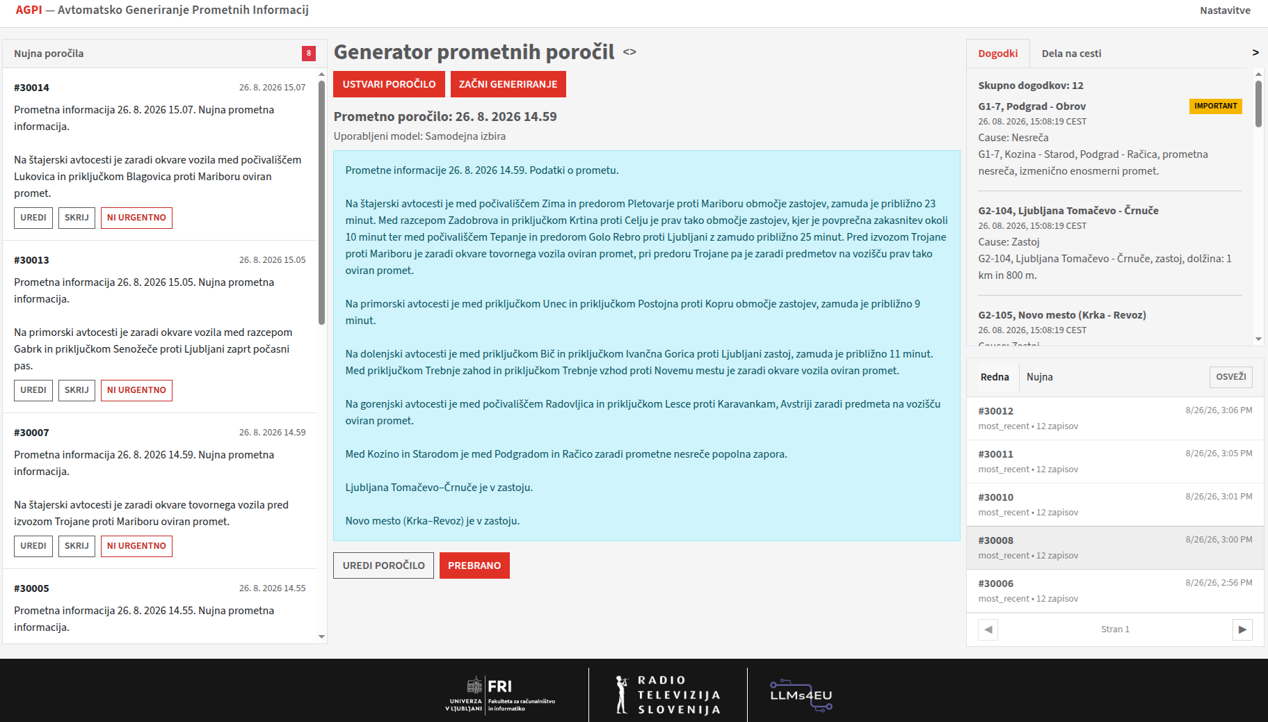
The left column lists urgent reports as they arrive, each with its own timestamp and generated text, and three actions: edit it, hide it, or mark it not urgent, letting an editor immediately flag a report that shouldn't have been fast-tracked in the first place, independent of whether its text was any good. The center panel shows the report currently being created or reviewed, including which model actually answered the call, automatic selection or a specific provider, matching provider_mode from Report Generation, alongside controls to generate a report and, once one exists, to edit or mark it read. The right column is split into two tabs: one lists the source events and roadworks a report can be built from, each with its road, cause, and description as fetched from NAP; the other lists recently created reports, kept in separate regular and urgent tabs.

An editor can mark a report's text as fine as-is, or leave detailed feedback: an edited version of the text, one or more flagged issue types, and a free-text comment, and a database constraint on the feedback record enforces that a plain "this is fine" can't quietly carry an edit or a comment alongside it, keeping the two kinds of feedback from blurring together. Urgent reports carry one more piece of feedback specific to them: whether the urgency call itself was right, not just the text, since an urgent report can be well-written and still have been the wrong report to fast-track in the first place.

The moment an editor saves an edited version of a report, that edited text becomes what everyone sees, not just that editor: the next person who opens the same report, no matter who they are, sees the latest edit instead of the model's original output.

Why This Matters

None of these decisions, splitting fetcher and transformer from the backend, giving the classifier its own service, pushing events over WebSocket instead of polling, or asking one Redis instance to do three jobs, exist because a bigger system needs more moving parts by default. Each one traces back to a real constraint this system actually has: a continuous background job that shouldn't compete with request handling, a differently-shaped workload on a different stack, a report whose entire value depends on reaching an editor immediately, a cost figure that only drops if repeat requests get answered from cache. Each split, each protocol choice, is a direct answer to one of those constraints, not a default assumption about what a "real" system needs.