AI-Based Image Analysis for Industrial Anomaly Detection and Quality Control

Overview

This computer-vision service helps manufacturing and quality-control teams train image-analysis models for visual product inspection. It covers the main steps needed for a specific product and image-acquisition setup: organising and annotating an image dataset, training the model, reviewing validation results, and applying the trained model to new production images. The current model supports supervised anomaly detection using labelled examples of acceptable and defective products together with pixel-level defect masks.

Outcome

The primary outcome is a trained visual anomaly-detection model adapted to the user's product and image-acquisition conditions. The service also produces the annotated image dataset and manifest used for training, recorded training parameters and model artifacts, validation metrics and visualisations, and inference results for new images. Inference results include an image-level anomaly score and a localisation map showing where the model detected unusual regions. These outputs support model validation and later integration into a visual quality-control process.

Service Card

Category	AI development and deployment
Domain	Visual Inspection, Quality Control
Vertical	Industry, Smart Manufacturing
Target users	Manufacturing Companies, Industrial SMEs, Industrial Automation Providers, Quality-Control and Production Teams
Service type	Self-Hosted AI Vision Service
Outputs	A trained visual anomaly-detection model, annotated image dataset and manifest, experiment records and model artifacts, validation metrics and visualisations, and inference results with anomaly scores and localisation maps.
Requirements	An x86-64 host with an NVIDIA GPU available to Docker, a representative production image dataset, and persistent local storage. Linux is supported directly. Windows 10 or 11 is supported through Docker Desktop using its WSL 2 backend and Linux containers. ARM and 32-bit x86 hosts are currently not supported. Supervised anomaly detection requires image-level acceptable/defective labels and a pixel-level defect mask for every defective image. Detailed hardware and image-data requirements are listed in the instructions.
Limitations	Performance depends on representative image data and stable image acquisition. Changes in product, camera, position, background, or illumination can reduce accuracy. The trained model and its decision threshold must be validated on production-representative images before operational use.
Availability	Q3/2026
Licensing	MIT License
Visual content
Visual caption

Using the service

This computer-vision service works with image datasets and runs on infrastructure managed by your organisation. Your images, annotations, trained models, validation results, and experiment records remain in the storage attached to the service.

The current supervised anomaly detection method learns from an image dataset containing labelled examples of acceptable and defective products. Defect masks show which image regions contain a defect. After training, the model can inspect new images, assign an anomaly score, and mark unusual regions.

The model is intended to support quality-control decisions. Before operational use, validate it on images collected under real operating conditions and select an appropriate decision threshold. Repeat validation whenever the product or image-acquisition setup changes.

The usual process is iterative:

1. Prepare the image dataset. Collect production-representative images and separate them into training and test sets.
2. Annotate the images. Add the labels, masks, or other annotations required by the selected method.
3. Train the model. Use the training set to create model weights.
4. Evaluate the model. Measure performance on the separate test set and inspect incorrect results.
5. Improve the data. Correct annotations, add missing examples, or collect more varied images, then train and evaluate again.
6. Use the final model. Save the selected model and run inference on new images, either in the service or through a deployed inference interface.

Most practical projects repeat steps 2–5 several times before the model is ready for deployment.

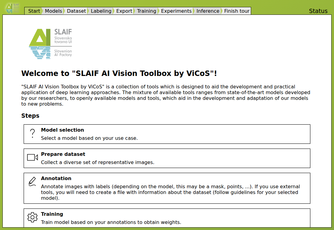
The guided tour keeps the complete process visible while you move through model selection, image-dataset preparation, training, experiments, and inference.

Supervised anomaly detection with SuperSimpleNet

Supervised anomaly detection trains a visual inspection model from a labelled image dataset of acceptable and defective products. Use one model for images that show the same product type from the same fixed view. Keep the camera, crop, scale, product position, background, and illumination consistent while including normal production variation.

This method uses SuperSimpleNet. The related paper is No Label Left Behind: A Unified Surface Defect Detection Model for all Supervision Regimes.

Required annotations and outputs

For the fully supervised setup described here, the image dataset must contain:

• acceptable and defective images of the same product and view;
• an image-level normal or abnormal label for every image;
• a pixel-level mask covering every defect in each defective image.

Acceptable images use an empty mask or no defect region. The mask should cover the defect without including harmless product texture or background.

For every inspected image, the trained model returns:

• an anomaly score that can be thresholded to classify the image as defective or non-defective;
• a pixel-level anomaly map that can be thresholded to segment the predicted defect.

The score is not a calibrated probability of a defect. You must validate the model and select a decision threshold for your production process.

Requirements

• an x86-64 host with an NVIDIA GPU (ARM and 32-bit x86 hosts are not supported);
• Docker with access to the GPU;
• persistent local storage for image datasets, service state, and model artifacts;
• representative training and test images with the labels and defect masks described above;
• stable image acquisition matching the intended operating conditions.

Deployment

Run this service on a computer or server managed by your organisation.

Host requirements

Requirement	Practical minimum for the documented example
Host platform	Linux x86-64, or Windows 10/11 x86-64 through Docker Desktop with its WSL 2 backend and Linux containers
Container runtime	Docker Engine 26.1 or later on Linux; a current Docker Desktop release on Windows
GPU runtime	Linux: NVIDIA Container Toolkit 1.14.5 or later with CDI enabled; Windows: Docker Desktop GPU support through WSL 2
NVIDIA driver	Linux: driver 580.95.05 or later, compatible with the current CUDA 13.0 Update 2 base image; Windows: a current NVIDIA driver with WSL 2 GPU support
Accelerator	NVIDIA GPU available inside Docker; 4 GB VRAM for training or 2 GB for inference
CPU	4 logical CPU cores
Host RAM	16 GB
Network	Internet access for the image download and first model installation
Browser	A current browser with access to the host
Port	Free TCP port 443 for the private web interface
Storage	At least 20 GB free, plus space for your image datasets and retained experiments
Shared memory	2 GB

The published container is a Linux x86-64 image. It can run on an x86-64 Windows host only through Docker Desktop's WSL 2 Linux-container backend; it is not a native Windows container. Run the documented shell commands from a WSL terminal and replace:

--device nvidia.com/gpu=all

with:

--gpus all

ARM hosts, including Windows on ARM, and 32-bit x86 hosts are currently not supported. The repository builds a Linux container from an NVIDIA CUDA Ubuntu base image, and the published image is available only for Linux x86-64.

The cell tile example was verified on a GeForce GTX 1080 Ti with 11 GB VRAM and NVIDIA driver 580.159.03. The current Toolbox Dockerfile uses the nvidia/cuda:13.0.3-cudnn-runtime-ubuntu24.04 base image. A direct CUDA memory check at 256×256 pixels measured about 2.05 GB reserved for a batch-4 training step and 262 MB for single-image inference. The 4 GB and 2 GB requirements include headroom for framework and worker overhead. Higher resolutions, larger batches, other backbones, concurrent workers, and other models require more GPU memory.

The 20 GB storage estimate allows for the published container image, the installed model environment, service state, and the prepared example. Production image datasets and retained MLflow runs require additional space.

Prepare persistent folders

mkdir -p \
  ~/slaif-ai-vision/datasets \
  ~/slaif-ai-vision/cache \
  ~/slaif-ai-vision/persist

These folders remain on the host after the container stops:

Host path	Container path	Contents
~/slaif-ai-vision/datasets	/data	Input datasets and exported annotations
~/slaif-ai-vision/cache	/cache	Downloaded model code and model environments
~/slaif-ai-vision/persist	/persist	Service settings, annotation projects, MLflow records, and trained artifacts

Copy every image dataset that you want to open in the service into ~/slaif-ai-vision/datasets. You can place each dataset in its own subfolder. For example:

cp -r /path/to/my-dataset ~/slaif-ai-vision/datasets/

The container sees the copied folder under /data. In this example, the corresponding container path is /data/my-dataset.

Pull the service image

The published image is available from Docker Hub:

docker pull vicoslab/slaif-ai-vision-toolbox:latest

The latest tag always downloads the current published version for Linux x86-64. The image download is approximately 4 GB.

Start the service

Do not expose the interface publicly

The current service does not provide user authentication. The command below binds the interface to 127.0.0.1. Do not expose ports 443 or 444 to the public internet.

docker run --rm -it \
  --name slaif-ai-vision \
  --publish 127.0.0.1:443:443 \
  --device nvidia.com/gpu=all \
  --shm-size=2g \
  --user "$(id -u):$(id -g)" \
  --volume ~/slaif-ai-vision/datasets:/data \
  --volume ~/slaif-ai-vision/cache:/cache \
  --volume ~/slaif-ai-vision/persist:/persist \
  --env "TOOLBOX_MODELS=W3sib3duZXIiOiJWaUNvUyIsImdyb3VwIjoiQW5vbWFseSBkZXRlY3Rpb24iLCJtb2RlbHMiOlsic3VwZXItc2ltcGxlLW5ldCJdLCJ1cmwiOiJodHRwczovL2dpdGh1Yi5jb20vdmljb3NsYWIvdG9vbGJveC1tb2RlbHMiLCAiYnJhbmNoIjogInNsYWlmIn1d" \
  vicoslab/slaif-ai-vision-toolbox:latest

Why TOOLBOX_MODELS is included

TOOLBOX_MODELS tells the service which compatible models to list when it starts for the first time. Its value is a Base64-encoded JSON list containing the model repository, branch, and model identifiers. The value in the command above loads super-simple-net from the slaif branch of https://github.com/vicoslab/toolbox-models and makes it available for installation.

You can replace the encoded value with another model-source string to offer a different compatible model or several models. This only changes which models are listed; users still choose which model to install.

The variable initializes the model-source configuration only when it does not already exist under /persist. When reusing an existing persistent folder, manage model sources from Models instead.

Allocate enough shared memory for training

Keep --shm-size=2g in the docker run command. If a training log reports a bus error, a failed data-loader worker, or insufficient shared memory, stop the container and start it again with a larger value, for example --shm-size=4g. This setting controls container shared memory, not GPU memory.

Open https://localhost. Your browser may warn about the local self-signed HTTPS certificate.

Install the model

The service currently uses the SuperSimpleNet model for supervised anomaly detection. Install it from the service interface:

1. Open Models.
2. Find SuperSimpleNet under Anomaly detection.
3. Select the install button and confirm.
4. Open Status and wait until the installation appears under Finished.

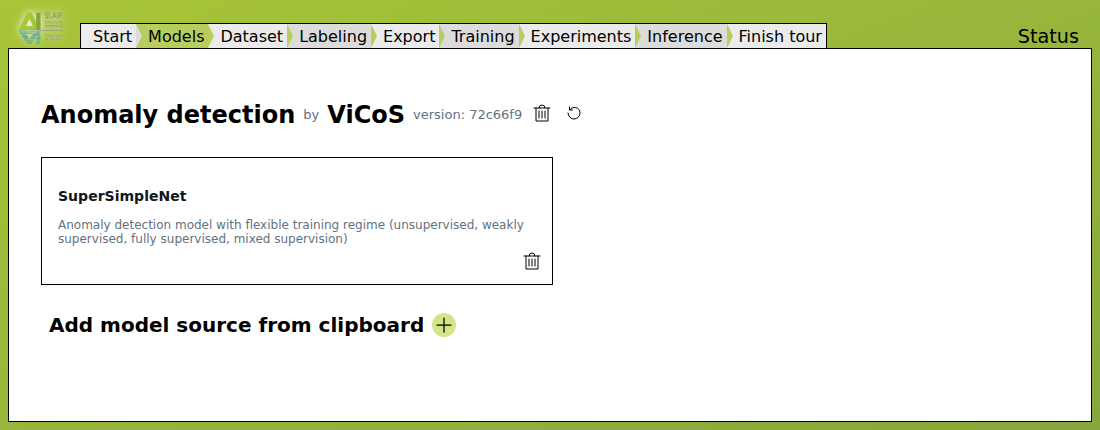
After installation, SuperSimpleNet appears under Anomaly detection. Open Status to confirm that installation finished successfully.

The first installation downloads the model environment and can take several minutes. If the task appears under Exited, open its log and report the last error to your administrator or service support contact.

Stop the service with Ctrl+C in the terminal. The three mounted folders preserve your work.

Training and monitoring with the cell tile example

The cell tile example is a prepared supervised dataset for checking one complete training cycle. It already contains labelled images, defect masks, and a manifest.json file. You do not need to annotate it.

The example confirms that the service can train the model, monitor the run, save the trained weights, and record validation results. It is not a production accuracy benchmark.

Complete the deployment steps above and install SuperSimpleNet before starting the cell tile example.

Download the example dataset

Download and extract cell-tile-demo.zip into the dataset folder created during deployment:

cd ~/slaif-ai-vision/datasets
curl --fail --location --remote-name https://data.vicos.si/slaif/cell-tile-demo.zip
unzip cell-tile-demo.zip

The ZIP extracts one flat directory named cell-tiles-demo:

~/slaif-ai-vision/datasets/cell-tiles-demo/
├── damaged_0_0000_ls3_camera0.jpg
├── damaged_0_0000_ls3_camera0_label.bmp
├── ...
├── okay_3_0025_ls3_camera0.jpg
├── okay_3_0025_ls3_camera0_label.bmp
└── manifest.json

The package contains 207 JPG images, 207 matching BMP masks, and one manifest. The manifest contains 103 abnormal and 104 normal examples. It uses a single data list, which SuperSimpleNet splits into 70% training and 30% test data when training starts. The split is stratified by label but is not currently fixed between runs.

Inside the service, the manifest is available at:

/data/cell-tiles-demo/manifest.json

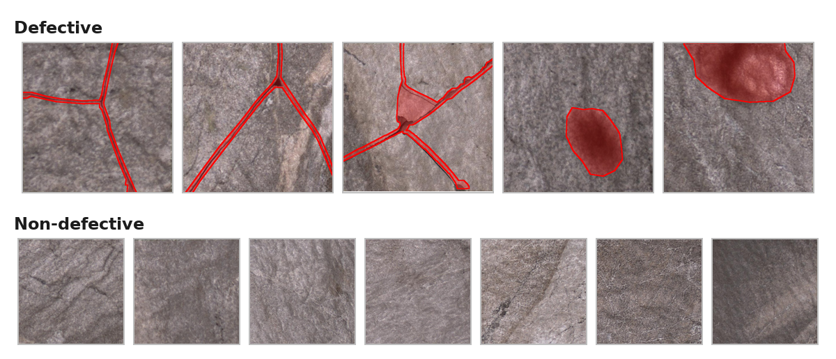
Defective samples with annotated regions shown in red (top), and non-defective samples (bottom).

Train the example

1. Open Models and select the installed SuperSimpleNet model.
2. At Dataset, select I have an external dataset.

3. In Training from external dataset, select the detected cell-tiles-demo/manifest.json. If it is not listed, enter:

   /data/cell-tiles-demo/manifest.json
   

   Do not forget to mount the dataset folder at /data

   The container can use the images only when the host dataset folder is mounted with --volume ~/slaif-ai-vision/datasets:/data in the docker run command. Without this mount, the container cannot read the manifest or training images.

4. Continue to Training. The Dataset manifest option is filled in automatically.

5. Under Model options, add Experiment name and enter Cell tile example.
6. Add Batch size and enter 4. Keep the image size at 256×256 pixels and Training duration at 10 epochs.
7. Select Start new. The service opens the task log while training runs.

Selecting an external manifest uses the prepared annotations directly for training. It does not create a Label Studio project.

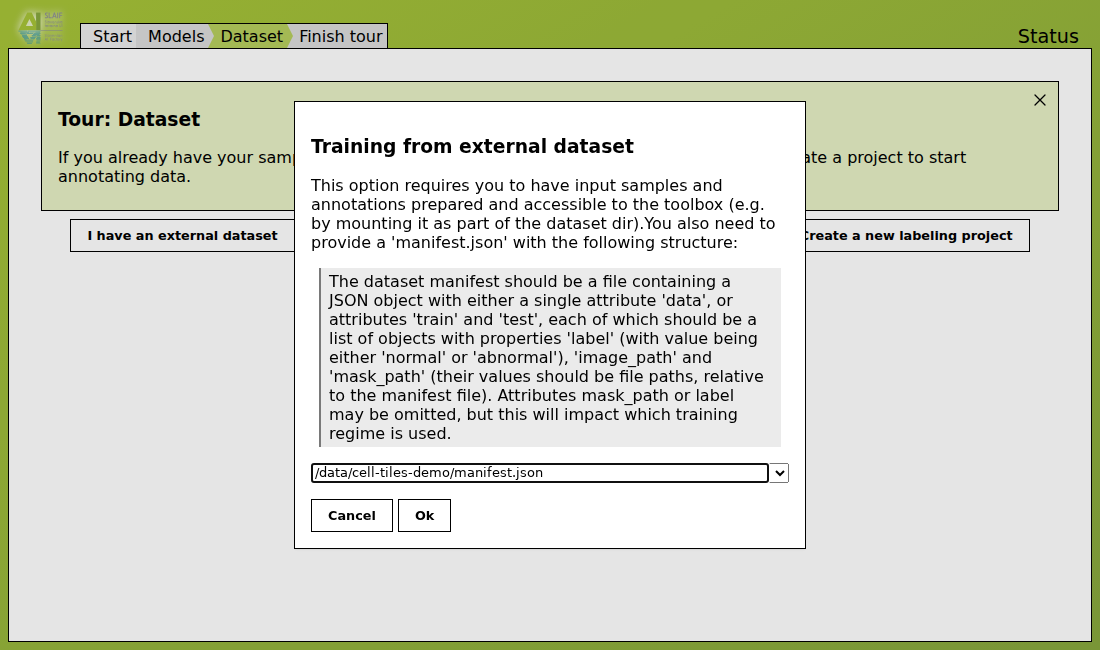
Select /data/cell-tiles-demo/manifest.json in the external dataset dialog.

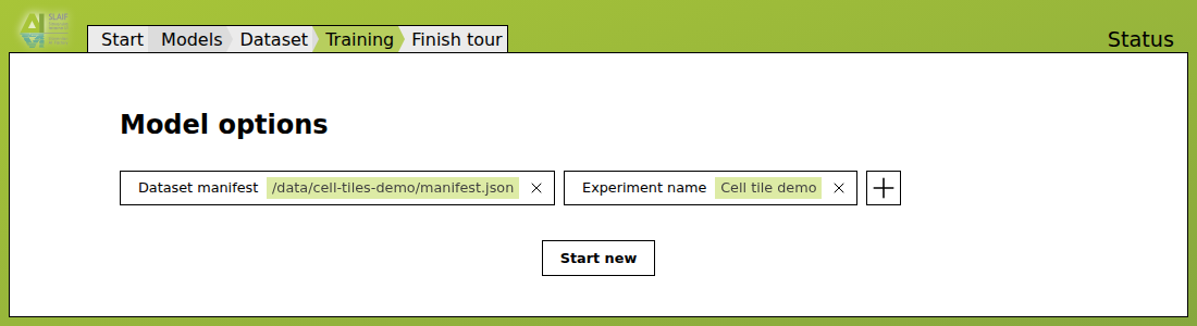
Check the manifest, give the run a clear name, and select Start new.

On the verified GTX 1080 Ti setup, this 10-epoch configuration completed in about 8 minutes. The reference run reduced avg_loss from 1.306 to 0.552 and achieved I-AUROC 0.922, P-AUROC 0.955, and AUPRO 0.816. On comparable hardware, allow approximately 7–10 minutes.

These values are a functional reference for one run with the supplied archive and documented settings, not a production guarantee. The automatic train/test split can vary between runs. Hardware, driver and library versions can also change runtime and results.

Monitor training

Follow the task on its log page. You can return to it through Status. Wait until the task finishes successfully. If it appears under Exited, inspect the last reported error.

Select Go to experiments on the task page, or open Experiments and then the SuperSimpleNet experiment. The completed run should contain:

• loss graphs under Model metrics;
• the parameters used for training;
• validation metrics;
• weights.pt, the trained model weights;
• results.json, the summary metrics;
• image_scores.json, the scores for individual validation images.

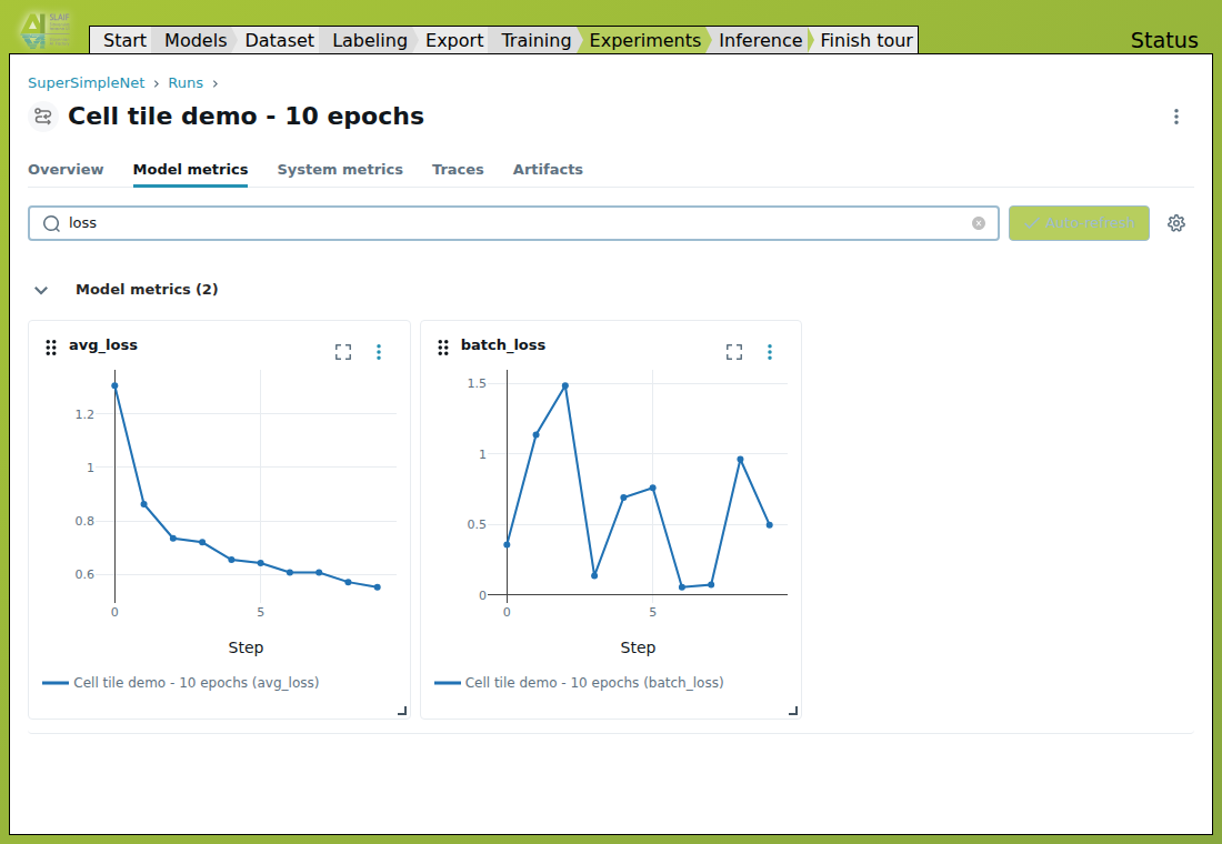
The completed example run in MLflow. Filtering by loss shows how avg_loss changes over the ten training epochs.

The training example is complete when the task finishes and weights.pt is present in the experiment.

Download the final outputs

Select Finish tour. The final page lists the cell tile dataset and the experiment artifacts associated with it, including the trained weights and evaluation outputs.

Use the download button next to Dataset or Experiment artifacts to download everything in that section. You can also expand folders and download an individual file or subdirectory. These are copies of the files kept in the mounted /data and /persist storage.

More advanced instructions

After completing the prepared example, continue with the instructions that match what you want to do next:

• Prepare and annotate your own image dataset — import production images, annotate them in Label Studio, and export the manifest expected by a model.
• Review experiments and artifacts — compare training runs, metrics, trained weights, and validation outputs in MLflow.
• Run inference and validate deployment — load trained weights, validate results on new images, and embed the inference-only interface in another webpage.
• Developing custom model — add a compatible model or extend an existing model module, training procedure, inference code, and service UI.

Prepare and annotate your own image dataset

The required annotations depend on the inspection method. A method may use only acceptable images, image-level acceptable/defective labels, defect masks, or a combination of these. Check the method page before annotating a large dataset.

Capture representative images

Use the same camera, lens, distance, product position, background, and illumination that you intend to use later. Include normal production variation, not only ideal samples.

Keep images of the same physical product or acquisition session in one data split. Near-duplicate images in both training and test sets can produce misleadingly good results.

Record at least:

• the product or batch identifier;
• the acquisition date and camera setup;
• whether the image is acceptable or defective, when required;
• the defect mask or other method-specific annotation, when required.

Formats and minimum dataset guidance

Data requirements depend on the selected model and its implementation. For the current SuperSimpleNet integration:

• use RGB JPEG, PNG, or TIFF images; the inference code converts input images to RGB;
• use a single-channel, lossless PNG or BMP mask with the same displayed width and height as its image;
• use value 0 for background and a non-zero value, normally 255, for defect pixels;
• do not use lossy JPEG files for masks;
• apply image orientation consistently to the image and mask before training.

The supplied example verifies JPG images with BMP masks. Label Studio exports masks as lossless .label.png files. Less common formats may work through the installed image readers, but should be tested before preparing a large dataset.

For the fully supervised setup and an automatically split data list, the technical minimum is two normal and two abnormal images so both classes can appear in the stratified training and test split. This is only enough to exercise the code. Current SuperSimpleNet training stops with an error when either split contains no normal samples. For a useful model, collect substantially more images and cover every product variant, acceptable production variation, defect type, size, position, and acquisition condition that the model must handle. The prepared demonstration uses 207 images: 104 normal and 103 abnormal.

If the manifest defines explicit train and test lists for supervised training, include normal and abnormal examples in both. At minimum, each split must contain a normal image. Keep images of the same physical item or acquisition sequence in one split.

Dataset manifest

Training uses a JSON manifest that lists images and their annotations. Paths are relative to the directory containing manifest.json. A common labelled example looks like this:

{
  "train": [
    {"image_path": "images/train/item-001.png", "label": "normal"},
    {
      "image_path": "images/train/item-017.png",
      "label": "abnormal",
      "mask_path": "masks/train/item-017.png"
    }
  ],
  "test": [
    {"image_path": "images/test/item-101.png", "label": "normal"}
  ]
}

Not every method uses every field. Use the manifest requirements stated on the selected method page.

Explicit train and test lists are recommended because they are easier to reproduce and audit. Keep the test set separate from data used to tune model options or a decision threshold.

If an annotated image dataset and manifest already exist under the mounted /data folder, select the model, open Dataset, and choose I have an external dataset. The service lists detected manifest.json files. Select one from the list or enter its full container path, then continue to Training. This uses the manifest directly and does not create a Label Studio project.

Annotate images in the service

1. Open Models and select the model you want to train.
2. At Dataset, select Create a new labeling project.
3. Choose the image directory under /data.
4. Review the selected images and the include or exclude file patterns, then create the project.
5. Open Labeling and select the first image.
6. Select the required label above the image, for example Anomaly. The selected label is used for the next annotation that you draw.
7. Select an annotation tool from the toolbar on the left. For a defect mask, use Brush, Magic Wand, or another mask tool provided by the project.
8. Draw the annotation on the image. Cover the defective region without including harmless texture or background.

9. Review the annotation and correct it if necessary. Press Submit for a new annotation, or Update when editing one, before moving to the next image. You must submit every image that should be used for training.

   Submit non-defective images too

   For anomaly detection, open each acceptable image and press Submit or Update without drawing a defect region. This records the image as normal. An unsubmitted image has no normal or abnormal label in the exported data and is ignored during training.

10. For each defective image, annotate every defective region and then submit it.

Annotation export is temporarily unavailable

The current Toolbox export worker does not refresh the status of Label Studio's asynchronous export job. It can wait until the five-minute timeout without creating manifest.json or providing Go to training. Until this is fixed in Toolbox, use an externally prepared manifest through Dataset → I have an external dataset. Your submitted Label Studio annotations remain stored in the project.

When creating the Label Studio project manually select the SLAIF anomaly-detection template

This service expects the prepared Anomaly Detection interface. Projects created through Dataset → Create a new labeling project receive the selected model's prepared interface automatically, so no extra setup is needed.

For a project created manually in Label Studio:

1. Open the project and go to Settings → Labeling Interface.
2. Select Browse Templates.
3. In the SLAIF AI Vision Toolbox by ViCoS template group, choose Anomaly Detection.
4. Select Save before importing or annotating images.

While creating a project directly in Label Studio, select the same template through Labeling Setup → Browse Templates. Do not use a generic image template because its labels and exported annotation format may not match the model.

Select label first, then tool

For each defect instance:

1. Select the label, for example Anomaly, by clicking it or pressing its number key on the keyboard.
2. Select the annotation tool on the left and draw the instance.
3. Press Esc to finish that instance.

Repeat all three steps for every additional instance: select the label, select the tool, draw, and press Esc when finished.

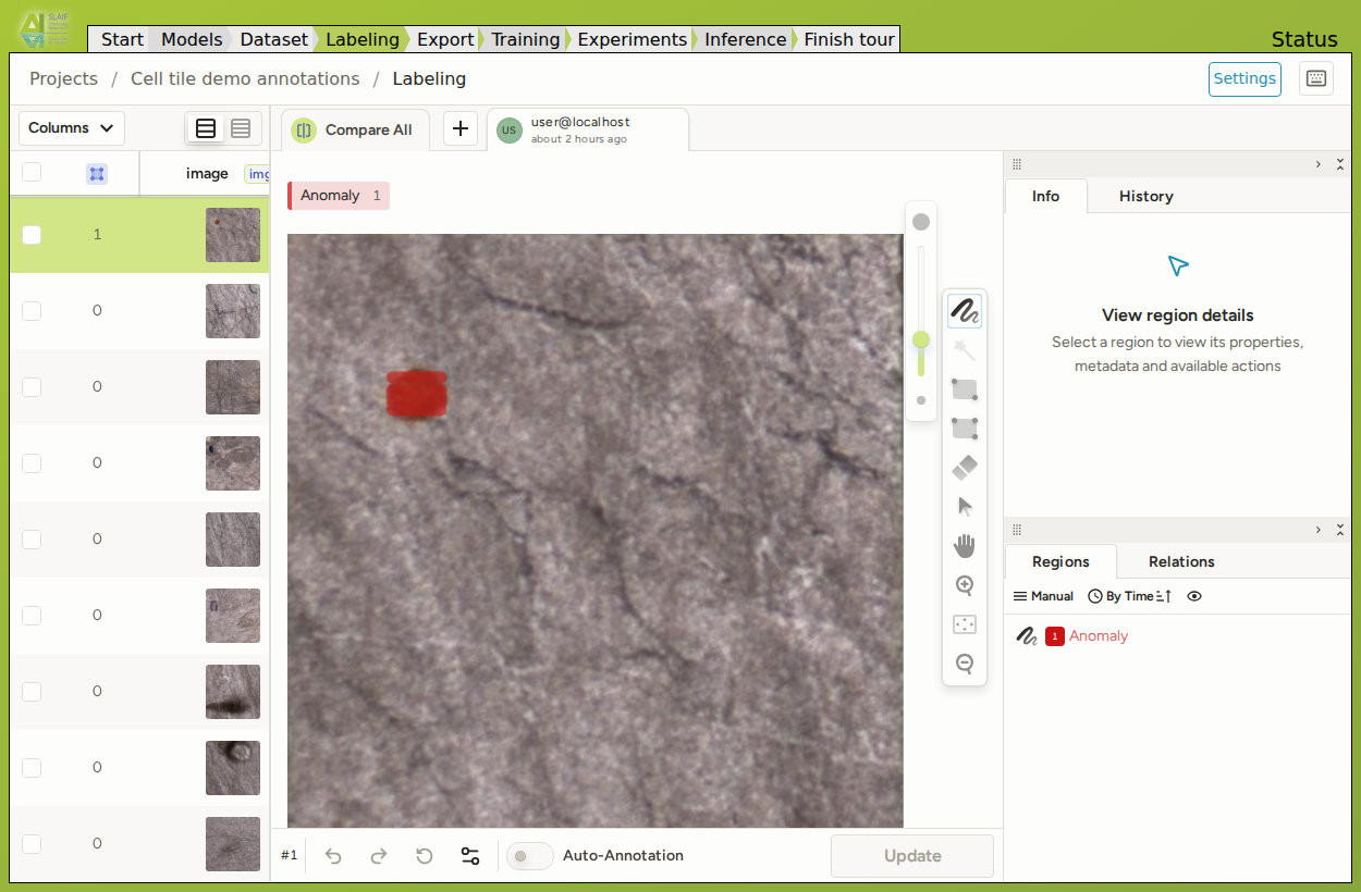
An anomaly mask after selecting the Anomaly label and Brush tool. Press Esc to finish the region before starting another one.

Customize the annotation interface

Label Studio defines an annotation interface with an XML configuration. The configuration specifies the displayed image, available labels, and tools such as brush masks, magic wand masks, rectangles, polygons, points, or other controls.

To view or edit the XML for the current Label Studio project:

1. Open the project in Labeling.
2. Select Settings → Labeling Interface.
3. Open the Code view.
4. Edit the XML and select Save.

This changes only the current Label Studio project. It does not change the prepared interface used by future projects.

For example, the current anomaly-detection configuration contains an Anomaly label and mask-oriented tools:

<View>
  <Labels name="labels" toName="image">
    <Label value="Anomaly" />
  </Labels>
  <Image name="image" value="$image" zoom="true" />
  <Brush name="brush" toName="image" />
  <MagicWand name="wand" toName="image" />
</View>

The model module supplies the default XML through the config: | block in its config.yml. For the current SuperSimpleNet integration, open super-simple-net/config.yml. Change this file when future projects created through the service should use a different interface. After publishing the change, open Models, select the refresh icon beside the model-source group, and confirm the update. The changed default is applied to newly created projects; update existing projects through Settings → Labeling Interface → Code.

You can add labels or another annotation tool, but the annotation format is part of the model contract. The export code and the model's training or inference code must understand the labels and geometry produced by the XML configuration. Changing only the XML can create annotations that the model cannot read.

When introducing a new annotation type:

1. Annotation interface: edit config.yml in the model module, or use Settings → Labeling Interface → Code for one existing project.
2. Annotation export: if the new Label Studio result type is not supported, update apps/ls-utils/export.py in the service-framework source. This is a code change; there is no setting for it in Label Studio.
3. Dataset manifest: define how the exported label or geometry is stored and update the model's documented manifest contract.
4. Training: update the model module's train.py or its dataset-loader helper to read the new manifest fields.
5. Inference and preannotation: update the model module's infer.py. Update ui.html if the new output should appear in the inference page, and update config.yml if Label Studio should display or receive the new annotation type.
6. End-to-end test: create an annotation, export it, train the model, and verify inference or preannotation with the new type.

Check the dataset before training

• Open a sample of images and annotations manually.
• Verify that every manifest path exists.
• Check labels, masks, or other method-specific annotations.
• Check that related images are not split between training and test data.
• Keep a copy of the exact manifest used for each reported result.

Review experiments and artifacts

The Experiments panel uses MLflow to record model training runs. The records and output files are stored in the host folder mounted at /persist.

Open a run

Training opens a task log page. Select Go to experiments there after the run has been created. You can also open Experiments, select the experiment created by the model, and choose a run by its name and start time.

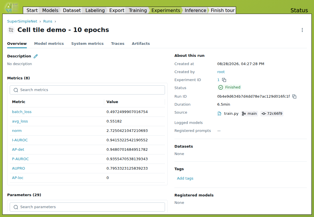
The run Overview collects its status, recorded metrics, training parameters, and links to metrics and artifacts.

A run normally records:

• the dataset and model options used for training;
• training and validation metrics;
• trained weights or checkpoints;
• method-specific evaluation files and visualisations.

Interpret metrics

Metric names depend on the selected method. Read the method documentation before comparing values. Compare runs only when they use the same dataset split and evaluation procedure.

Filter the charts by loss to inspect the training curve. In this 10-epoch example, avg_loss decreases steadily while individual batch losses vary.

Do not select a model from one metric alone. Review missed defects, false rejections, localisation results, and examples captured under realistic operating conditions.

Artifacts

Artifacts are the files saved by a training run. They can include:

• trained model weights or checkpoints;
• summary metrics;
• scores for individual validation images;
• localisation maps or other visualisations;
• configuration files needed to reproduce the run.

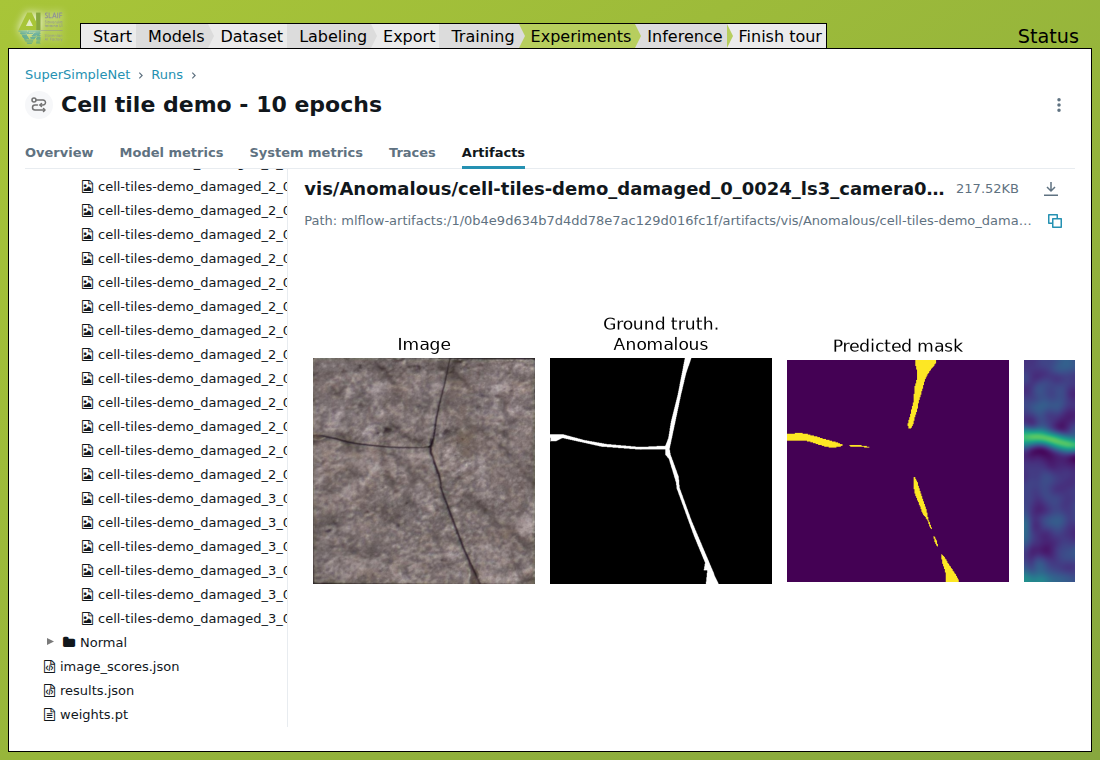
The artifact tree contains the trained weights.pt model and validation outputs. Here, an abnormal sample visualization shows the image, ground truth, predicted mask, and anomaly map.

Artifact names vary by model. Use Go to inference when the completed task provides it. Otherwise open the model's inference page, add its weights or checkpoint option under Model options, and select an artifact from the listed MLflow runs.

Back up the complete /persist folder. Model weights without their dataset manifest, parameters, and evaluation record are difficult to reproduce or audit.

Compare runs fairly

When changing a training option:

• keep the same training and test split;
• keep the same random seed when the model provides one;
• change one main option at a time;
• give each run a descriptive name;
• record why you selected the final run.

Run inference and validate deployment

Inference applies a trained model to images that were not used for training. The inputs and result display depend on the selected model.

Start inference

1. Open the completed training task and select Go to inference. The new weights may be filled in automatically.
2. Alternatively, open the model's inference page, add its weights or checkpoint option under Model options, and select an artifact from a past MLflow run.
3. Optionally add Alias under Model options. The alias names the worker and becomes the last part of its /infer/<alias> URL. Each active worker must have a unique alias. If no alias is set, the model identifier is used.
4. Select Start new. The page reloads and shows the active worker in an expandable panel.
5. Open the worker panel, upload one or more images, and review the returned results. Use the remove button in the panel when you want to stop that worker.

Review the outputs defined by the selected model. They may include scores, localisation overlays, masks, counts, classes, or other method-specific results.

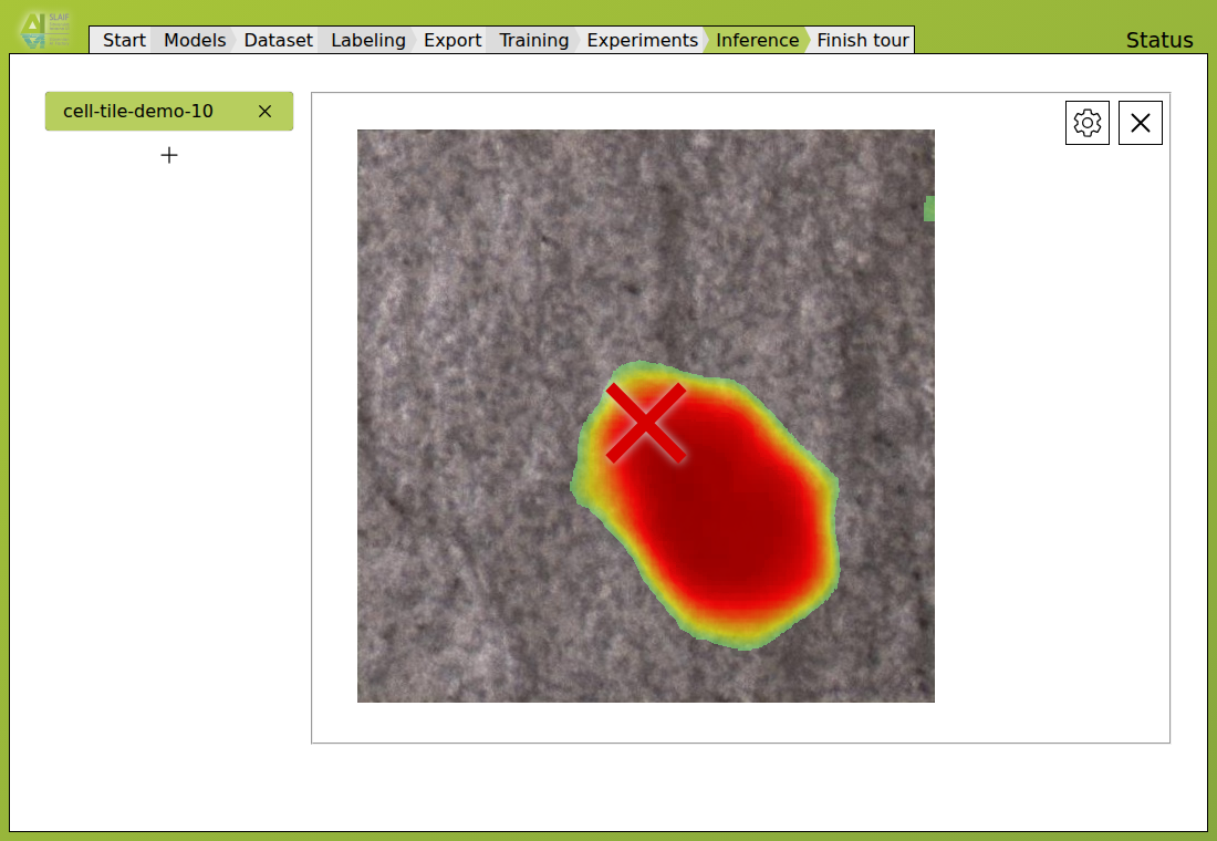
The cell-tile-demo-10 worker localizes a visible defect in damaged_3_0005_ls3_camera0.jpg, an image from the run's training split.

Validate the result

Before using inference for an operational decision:

1. choose a threshold or decision rule on a separate validation set, when the method requires one;
2. count missed defects and false rejections;
3. review results separately for each product variant and defect type;
4. inspect both correct and incorrect decisions;
5. agree on what happens when the service is unavailable or the result is uncertain.

Repeat validation after any change to the product, camera, lens, position, background, illumination, or image processing.

Embed the inference interface in a webpage

The service provides a standalone page for each active inference model:

https://YOUR-INFERENCE-HOST/infer/MODEL-ALIAS

This page contains only the model-specific inference interface. It does not expose dataset annotation, training, experiment tracking, or model-management pages. It can therefore be embedded into another website with an iframe:

<iframe
  src="https://YOUR-INFERENCE-HOST/infer/MODEL-ALIAS"
  title="AI visual inspection"
  style="width: 100%; min-height: 720px; border: 0;"
  loading="lazy">
</iframe>

The embedded page is available while its inference worker is active. Several workers can run at the same time when each uses a different alias.

Start an iframe worker on demand

For a production-facing iframe, TOOLBOX_AUTOSTART can map a public alias to a model and its inference options. A request to that alias starts the worker when it is not already active:

--env 'TOOLBOX_AUTOSTART={"quality-control":{"model":"super-simple-net","config":{"weights":"/persist/mlflow/artifacts/EXPERIMENT_ID/RUN_ID/artifacts/weights.pt"}}}'

Replace the weights path with a trained file that exists inside the container. The model must already be installed in the persistent /cache folder. With this example, embed:

https://YOUR-INFERENCE-HOST/infer/quality-control

An automatically started worker is stopped after approximately 15 minutes without requests. A later request starts it again.

Expose the inference endpoint

To publish the separate inference endpoint, add this mapping to docker run:

--publish 127.0.0.1:444:444

Replace the localhost binding only when an administrator has placed the endpoint behind appropriate TLS, authentication, and other access controls. The public endpoint currently limits each client to one inference request every 5 seconds and 100 inference requests per day. These limits do not provide authentication and may not match the capacity or policy of your deployment. Embedding the inference page does not secure it by itself.

To record requests that reach the public inference endpoint, add:

--env TOOLBOX_ACCESS_LOG=/persist/toolbox/access.log

The log records the endpoint alias, client address, time, and submitted filenames. The current file is recreated when the service starts.

Developing custom model

The service framework can use any image-analysis model that implements its model-module contract. You can add a new model or extend an existing module with different inputs, annotations, training options, outputs, or interface elements.

Start from the current module sources:

Browse the SLAIF model modules on GitHub

The repository contains several model modules that can be used as working examples. Any of them can be extended or used as the starting point for a new compatible model. This page uses defect-type classification with SuperSimpleNet as one possible example; that extension is not a released feature.

How the model module connects to the service

The service discovers a model from a directory containing a small set of conventional files. The SuperSimpleNet module provides one complete reference:

File	Role in the service
model.json	Defines the model name, description, and options shown under Model options. Descriptions are available by hovering over an option. The same values are converted to command-line arguments for training and inference. File formats also control manifest and MLflow-artifact suggestions.
config.yml	Defines the annotation project used for anomaly masks.
setup.sh	Downloads the upstream model code, applies patches, creates its Python environment, and installs dependencies. The Install action runs this script.
train.py	Reads the manifest and model options, trains and evaluates the model, logs parameters and metrics to MLflow, and saves artifacts such as weights.pt. Start new on the Training page runs this script and opens its task log.
infer.py	Loads trained weights and implements command-line, HTTP, and annotation-backend inference. Start new on the Inference page starts this module as a named worker.
ui.html	Defines the inference-only browser interface. It uploads images and displays returned scores and anomaly maps. The same fragment is used in each active-worker panel and the standalone /infer/<alias> page.
Patch files	Adapt upstream dependencies and visualisation code to the service environment and MLflow artifact logging.

Use "format": "file:manifest.json" for a manifest option so the Dataset and Training pages can discover manifests under /data. Use a file format such as "file:weights.pt" for trained weights so the Inference page can list matching artifacts from MLflow runs. The service itself adds the optional Alias field used to distinguish multiple active inference workers; it does not need to be declared in model.json.

Example: add defect-type classification

The following sections show one possible extension to SuperSimpleNet. The standard module returns an anomaly score and an anomaly map. This example also returns the most likely defect type for images classified as defective. A different model or extension can define another dataset contract, training procedure, and output interface.

Extend the dataset contract

Add defect_type to defective examples:

{
  "image_path": "images/train/item-017.png",
  "label": "abnormal",
  "mask_path": "masks/train/item-017.png",
  "defect_type": "scratch"
}

Use a fixed class list, for example scratch, dent, and stain. If one image can contain several types, use a multi-label output instead of the single-class design shown here.

Update the training data loader to:

• reject unknown defect types;
• map class names to stable integer IDs;
• train the classifier only on defective images with a known type;
• store the class-name mapping with the model artifacts.

Add model options to the UI

Add the class list and any classification settings to model.json. The service automatically exposes these options under Model options and forwards the selected values to train.py and infer.py.

A simple string option can hold a fixed class list:

"defect_types": {
  "title": "Defect types",
  "description": "Comma-separated class names in a fixed order.",
  "type": "string",
  "default": "scratch,dent,stain"
}

Use the same option names in the training and inference code. If the extension needs a richer input type that model.json cannot represent, the service UI must be extended as well.

Extend training and saved artifacts

train.py is the model-specific training entry point and the bridge between the generic service interface and the underlying SuperSimpleNet implementation. When the user selects Start new, the service reads the selected values, converts them to command-line arguments, starts train.py, and displays its task log. The framework does not implement the model's learning procedure.

Together, model.json and train.py define the complete training contract:

• model.json declares which parameters are available under Model options, their types, descriptions, and default values;
• train.py reads those values and defines what they do;
• it loads and checks the manifest, creates or uses the training and test split, and determines the supervision regime;
• it constructs the data loaders and model, then controls preprocessing, losses, optimization, training duration, and model saving;
• it defines when validation runs, which metrics are calculated, and which visualisations and JSON summaries are produced;
• it records parameters and metrics in MLflow and saves artifacts such as weights.pt.

A new training option therefore normally requires changes in both places: expose it in model.json, then implement and use it in train.py. Changes to validation, metrics, or saved artifacts belong in train.py; Toolbox will display the resulting logs and MLflow records without implementing that model-specific logic itself.

For defect-type classification, update train.py to:

1. obtain image features from the model or from the predicted defect region;
2. add a classification head;
3. combine its loss with the existing anomaly-detection losses;
4. log classification metrics to the current MLflow run;
5. save the head, class mapping, and other required configuration with the trained weights.

Do not classify from the single anomaly score alone. Report macro F1, per-class precision and recall, and a confusion matrix. Keep the original anomaly metrics so that the extension can be compared with the standard model.

Extend inference and the inference page

Update infer.py to return the defect type and its score alongside the existing outputs:

{
  "scores": [0.91],
  "anomaly_maps": ["..."],
  "defect_types": ["scratch"],
  "defect_type_scores": [0.82]
}

Update ui.html to display the type only when the anomaly score passes the validated anomaly threshold. Because ui.html is also used by the standalone inference page, this change appears both in the service and in an iframe deployment.

If annotation-assisted prediction should include the defect type, update the annotation response generated by infer.py and make sure config.yml contains matching labels.

Package and test the customized module

Create a separate model directory, for example super-simple-net-defect-types, rather than changing the released module in place. Then:

1. update setup.sh if the classifier requires extra dependencies;
2. publish the new model directory in a Git repository;
3. register it through the model-source JSON process described below;
4. install it through Models;
5. test training from a manifest containing all configured defect types;
6. test loading the saved weights in a new inference worker;
7. test the full model page and the standalone iframe page;
8. confirm that anomaly-only results still work when defect classification is not requested.

Register a custom model source

A model source is registered with a Base64-encoded JSON list, either through TOOLBOX_MODELS during first initialization or through Add model source from clipboard. The service reads model.json and ui.html from the registered source before installation. It enables training when train.py is present. Installation remains separate and runs setup.sh only when the user selects Install.

The source-registration JSON is separate from the model.json file inside each model directory. It tells the service which Git repository and model directories to load. For example:

[
  {
    "owner": "My organisation",
    "group": "Defect detection models",
    "models": [
      "super-simple-net-defect-types"
    ],
    "url": "https://github.com/my-organisation/toolbox-models",
    "branch": "main"
  }
]

• owner and group are displayed on the Models page;
• every value in models must match a model directory in the repository;
• url is the Git repository containing those directories;
• branch selects the branch to clone. Use the branch that contains the published model modules; omit it only when the repository's default branch is correct.

On Linux, save and encode the JSON with:

cat > model-source.json <<'JSON'
[
  {
    "owner": "My organisation",
    "group": "Defect detection models",
    "models": ["super-simple-net-defect-types"],
    "url": "https://github.com/my-organisation/toolbox-models",
    "branch": "main"
  }
]
JSON

python3 -m json.tool model-source.json > /dev/null
base64 -w 0 model-source.json > model-source.b64
cat model-source.b64

The first command writes the JSON, the second checks its syntax, and the final two commands create and display the Base64 string. To check the encoded file:

base64 --decode model-source.b64 | python3 -m json.tool

Copy the single-line contents of model-source.b64. On an existing service, copy it to the clipboard, open Models, select Add model source from clipboard, and confirm. For first initialization, place the same string in the TOOLBOX_MODELS value passed to docker run.

Using an online Base64 encoder

You can paste the model-source JSON into an online Base64 encoder and copy its encoded output. Base64 is not encryption: do not include passwords, access tokens, private repository credentials, or other secrets. Check the decoded JSON before importing it.